Introduction

对比学习是一种为机器学习模型描述相似和不同事物的任务的方法。它试图教机器区分相似和不同的事物。

对比学习框架

• 对比学习不需要标签，自动就能学。
• 不是分类任务
• 目标是判断是不是同一个（是不是自己），自己与自己互为正样本，自己与其它互为负样本
• 训练时是需要负样本的，不然可能会导致模型坍塌
• 对比学习可以用来提特征
• 对比学习相比有监督的学习，其泛化能力更强一些

Sourece Codes

• https://github.com/lucidrains/DALLE2-pytorch

Papers

2020 SimCLR

[1] T. Chen, S. Kornblith, M. Norouzi, and G. Hinton, A Simple Framework for Contrastive Learning of Visual Representations, Jun. 30, 2020, arXiv: arXiv:2002.05709. https://github.com/google-research/simclr

Introduction

      蒙特卡洛定位算法（Monte Carlo Localization, MCL）的公式推导涉及粒子滤波（Particle Filter）的数学基础。粒子滤波是一种基于递归贝叶斯估计的方法，用于对系统状态进行估计。其基本目标是根据传感器观测和运动模型来估计机器人的位置和姿态。

Angent的实现

Overview

之前学习了状态迁移函数，并能绘制机器人。

这节的目标是实现机器人的引擎，让机器人能动起来。

笔记

• ロボットの制御指令を決めるエージェントのクラスを作ります。
• 「考え主体」のことを、ロボチックスや人工知能の研究分野ではエージェントと呼びます。
• 今の段階ではただ一定自家ごとに固定値の$\nu, \omega$を返すというもとにします。
• hasattrは、オブジェクトにメソッドがあるかを調べる関数です。
• 何秒間シミュレーションするか(time_span) と$\Delta t$ (time_interval)を指定できるようにします。

理论

• 机器人通过机器人来发布控制指令。
• 控制指令： $\nu = (\nu, \omega)^\top$
• 设定仿真时长(time_span)，第帧的时间间隔(time_interval)
• 帧数 = time_span/time_interval
• hasattr用来检查对象是否存在

Sample Code

# -*- coding: utf-8 -*-
"""ch3 robot model

Automatically generated by Colaboratory.

Original file is located at
    https://colab.research.google.com/drive/1s6LUufRD3f70hqtnyt9tsTqXnEJN7QL1
"""

# Commented out IPython magic to ensure Python compatibility.
# %matplotlib inline
import matplotlib.pyplot as plt
import matplotlib.patches as patches
import math
import numpy as np

# Animation
import matplotlib
matplotlib.use('nbagg')
import matplotlib.animation as anm
from matplotlib import rc

"""# Draw world coordinate"""

class World:
  def __init__(self, time_span, time_interval, debug=False):
    self.objects = []
    self.debug = debug
    self.time_span = time_span
    self.time_interval = time_interval

  def append(self, obj):
    self.objects.append(obj)
  
  def draw(self):
    global ani
    fig = plt.figure(figsize=(4, 4))
    plt.close()
    ax = fig.add_subplot(111)
    ax.set_aspect('equal')
    ax.set_xlim(-5, 5)
    ax.set_ylim(-5, 5)
    ax.set_xlabel("X", fontsize=20)
    ax.set_ylabel("Y", fontsize=20)

    elems = []

    if self.debug:
      for i in range(1000):
        self.one_step(i, elems, ax)
    else:
      ani = anm.FuncAnimation(fig, self.one_step, fargs=(elems, ax), frames=int(self.time_span/self.time_interval)+1, interval=int(self.time_interval*1000), repeat=False )
      plt.show()


  def one_step(self, i, elems, ax):
    while elems: elems.pop().remove()
    elems.append(ax.text(-4.4, 4.5, "t="+str(i), fontsize=10) )
    for obj in self.objects:
      obj.draw(ax, elems)
      if hasattr(obj, "one_step"): obj.one_step(1.0)

class Agent:
  def __init__(self, nu, omega):
    self.nu = nu
    self.omega = omega

  def decision(self, observation=None):
    return self.nu, self.omega

"""# Robot Object"""

class IdealRobot:
  def __init__(self, pose, agent=None, color="black"):
    self.pose = pose
    self.r = 0.2
    self.color = color
    self.agent = agent
    self.poses = [pose]

  def draw(self, ax, elems):
    x, y, theta = self.pose
    xn = x + self.r * math.cos(theta)
    yn = y + self.r * math.sin(theta)
    elems += ax.plot([x, xn], [y, yn], color=self.color)
    c = patches.Circle(xy=(x,y), radius=self.r, fill=False, color=self.color)
    elems.append(ax.add_patch(c))

    self.poses.append(self.pose)
    elems+=ax.plot( [e[0] for e in self.poses], [e[1] for e in self.poses], linewidth=0.5, color="black")
  @classmethod
  def state_transition(cls, nu, omega, delta_t, pose):
    theta_t_pre = pose[2]
    if math.fabs(omega) < 1e-10:
      return pose + np.array([nu * math.cos(theta_t_pre),
                                  nu * math.sin(theta_t_pre),
                                  omega
      ]) * delta_t
    else:
      return pose + np.array([  nu/omega * (math.sin(theta_t_pre + omega * delta_t) - math.sin(theta_t_pre)),
                              nu/omega * (-math.cos(theta_t_pre + omega * delta_t) + math.cos(theta_t_pre)),
                              omega * delta_t
      ])
  
  def one_step(self, time_interval):
    if not self.agent: return
    nu, omega = self.agent.decision()
    self.pose = self.state_transition(nu, omega, time_interval, self.pose)

# Commented out IPython magic to ensure Python compatibility.
# %matplotlib inline
world = World(time_span = 36, time_interval = 1, debug=False)

straight = Agent(0.2, 0.0)
circling = Agent(0.2, 10.0/180*math.pi)
robot1 = IdealRobot(np.array([1, 1, math.pi/6]).T, straight)
robot2 = IdealRobot(np.array([-2, -1, math.pi/5*6]).T, circling, "red")
robot3 = IdealRobot(np.array([0, 0, 0]).T, color="blue")
world.append(robot1)
world.append(robot2)
world.append(robot3)

world.draw()

# this is needed to show animation whithin colab
rc('animation', html='jshtml')
ani    # or HTML(anim.to_jshtml()

Graphrag

Graphrag是什么?

GraphRAG 是一种结构化的、分层的检索增强生成（RAG）方法，而不是使用纯文本片段的语义搜索方法。GraphRAG 过程包括从原始文本中提取出知识图谱，构建社区层级(这种结构通常用来描述个体、群体及它们之间的关系，帮助理解信息如何在社区内部传播、知识如何共享以及权力和影响力如何分布)，为这些社区层级生成摘要，然后在执行基于 RAG 的任务时利用这些结构。

Introduction

Prepare Camera and Lidar

• Start Lidar

roslaunch pepperl_fuchs_r2000 r2000.launch scanner_ip:=192.168.3.1

topic name: /r2000_node/scan

• Start USB camera

roslaunch usb_cam usb_cam-test.launch

or

roslaunch usb_cam.launch dev:=/dev/video4

usb_cam.launch:

<launch>
    <arg name="dev" default="/dev/video0" />
  <node name="usb_cam" pkg="usb_cam" type="usb_cam_node" output="screen">
    <param name="video_device" value="$(arg dev)" />
    <param name="image_width" value="640" />
    <param name="image_height" value="480" />
    <param name="pixel_format" value="yuyv" />
    <param name="camera_frame_id" value="usb_cam" />
    <param name="io_method" value="mmap"/>
  </node>
</launch>

topic name: /usb_cam/image_raw

Objective

• 绘制世界坐标系
• 如何描述机器人的位姿
• 如何绘制世界坐标系
• 如何绘制机器人位姿

可参考：3.2.2 ロボットの姿勢と描く

対向２輪ロボット(Differential wheeled robot)

机器人位姿

• 世界坐标系记为 $\Sigma_{world}$

• 位姿 (状态)：位置和朝向 $x = (x, y, \theta)^T$

  %%Objective 绘制世界坐标系 如何描述机器人的位姿 如何绘制世界坐标系 如何绘制机器人位姿 可参考：3.2.2 ロボットの姿勢と描く 対向２輪ロボット(Differential wheeled robot) 机器人位姿 世界坐标系记为 $\Sigma_{world}$ 位姿 (状态)：位置和朝向 $x = (x, y, \theta)^T$ 状态空间： 姿势（状态）的集合 位姿x所有可能的取值的集合$\chi$，例如平面上的长方形的范围内自由移动的机器人位姿的状态空间为： $$ \chi = { x=(x, y, \theta)^T | x \in [x_{min}, x_{max}], y \in [y_{min}, y_{max}], \theta \in [- \pi, \pi) } $$ Source Code import matplotlib.pyplot as plt import matplotlib.patches as patches import math import numpy as np class World: def __init__(self): self.objects = [] def append(self, obj): self.objects.append(obj) def draw(self): fig = plt.figure(figsize=(8, 8)) ax = fig.add_subplot(111) ax.set_aspect('equal') ax.set_xlim(-5, 5) ax.set_ylim(-5, 5) ax.set_xlabel("X", fontsize=20) ax.set_ylabel("Y", fontsize=20) for obj in self.objects: obj.draw(ax) plt.show() class IdealRobot: def __init__(self, pose, color="black"): self.pose = pose //位姿 self.r = 0.2 // 半径 self.color = color // 顡色 def draw(self, ax): x, y, theta = self.pose xn = x + self.r * math.cos(theta) yn = y + self.r * math.sin(theta) ax.plot([x, xn], [y, yn], color=self.color) c = patches.Circle(xy=(x,y), radius=self.r, fill=False, color=self.color) ax.add_patch(c) world = World() robot1 = IdealRobot(np.array([2, 3, math.pi/6]).T) robot2 = IdealRobot(np.array([-2, -1, math.pi/5*6]).T, "red") world.append(robot1) world.append(robot2) world.draw() References 詳解　確率ロボティクス　Ｐｙｔｈｏｎによる基礎アルゴリズムの実装 $$$ 机器人开发环境介绍%%//milaiai.com:1313/post/ch1-environment/%%2025-07-10%%

  机器人开发环境介绍

  In this section, we will tintroduce:

  1. the usage case of robots
  2. the development environment for simulation (Python + conda)

  概率机器人详解

  概率机器人详解 Homepage

  课件: ryuichiueda/LNPR_SLIDES

  原书代码: ryuichiueda/LNPR_BOOK_CODES

  My source code: https://github.com/yubaoliu/Probabilistic-Robotics.git

  Robot Introduction

  Soccer match:

  Human support robot:

  Note: you can find these videos on https://space.bilibili.com/52620240 too.

  Environment Deployment

  • (optional) Anyconda or other virtual Python environment
  • Jupyter notebook

  You can refer https://www.ybliu.com/2021/01/OpenCV-Python-Development.html to deploy a conda-based development environment.

  %%机器人开发环境介绍 In this section, we will tintroduce: the usage case of robots the development environment for simulation (Python + conda) 概率机器人详解 概率机器人详解 Homepage 课件: ryuichiueda/LNPR_SLIDES 原书代码: ryuichiueda/LNPR_BOOK_CODES My source code: https://github.com/yubaoliu/Probabilistic-Robotics.git Robot Introduction Soccer match: Human support robot: Note: you can find these videos on https://space.bilibili.com/52620240 too. Environment Deployment (optional) Anyconda or other virtual Python environment Jupyter notebook You can refer https://www.ybliu.com/2021/01/OpenCV-Python-Development.html to deploy a conda-based development environment. Test Environment Run jupyter notebook jupyter notebook Add vitual env to notebook: conda install -c anaconda ipykernel python -m ipykernel install --user --name=robotics jupyter notebook Draw world coordinate Source code: import matplotlib.pyplot as plt class World: def __init__(self): pass def draw(self): fig = plt.figure(figsize=(8, 8)) ax = fig.add_subplot(111) ax.set_xlim(-5, 5) ax.set_ylim(-5, 5) ax.set_xlabel("X", fontsize=20) ax.set_ylabel("Y", fontsize=20) plt.show() world = World() world.draw() $$$ 机器人概率基础%%//milaiai.com:1313/post/ch2-probabilistics/%%2025-07-10%%

  

  平均値

  $$\mu = \frac{1}{N}\sum_{i=0}^{N-1} z_i$$

  • $z_0, z_1, \dots, z_{N-1}$: センサ値
  • $N$: センサ値の個数

  分散、標準偏差

  $$\sigma^2 = \frac{1}{N-1}\sum_{i=0}^{N-1} (z_i - \mu)^2 \quad (N>1)$$

  (素朴な）確率分布

  ここでやりたいこと: 度数分布から、 未来にどんなセンサ値が得られそうかを予想

  • ただし、集める個数によって値が変わってはいけないので度数分布を頻度でなく割合に * $P_{\textbf{z}\text{LiDAR}}(z) = N_z / N$　（$N_z$: センサの値が$z$だった頻度） * 全センサ値の種類に関して$P_{\textbf{z}\text{LiDAR}}(z)$を足し合わせると1に $P_{\textbf{z}\text{LiDAR}}(z)$を確率と呼びましょう

  Samples

  draw:

  %% 平均値 $$\mu = \frac{1}{N}\sum_{i=0}^{N-1} z_i$$ $z_0, z_1, \dots, z_{N-1}$: センサ値 $N$: センサ値の個数 分散、標準偏差 $$\sigma^2 = \frac{1}{N-1}\sum_{i=0}^{N-1} (z_i - \mu)^2 \quad (N>1)$$ (素朴な）確率分布 ここでやりたいこと: 度数分布から、 未来にどんなセンサ値が得られそうかを予想 ただし、集める個数によって値が変わってはいけないので度数分布を頻度でなく割合に * $P_{\textbf{z}\text{LiDAR}}(z) = N_z / N$　（$N_z$: センサの値が$z$だった頻度） * 全センサ値の種類に関して$P_{\textbf{z}\text{LiDAR}}(z)$を足し合わせると1に $P_{\textbf{z}\text{LiDAR}}(z)$を確率と呼びましょう Samples draw: $$ z \sim P_{\textbf{z}\text{LiDAR}} $$ Probabilistic Model ガウス分布の当てはめ 连续的情况 $$ p(z | \mu, \sigma^2 ) = \frac{1}{\sqrt{2\pi}\sigma} e^{ - \frac{(z - \mu)^2}{2\sigma^2}} $$ $$ p(x | \mu, \sigma^2 ) $$ $\mu$: 平均値、$\sigma$: 標準偏差 確率密度関数 Probability Density Function, PDF ガウス分布からの確率の求め方: $p(x | \mu, \sigma^2 )$を積分 $p$の値を密度と言う 密度を積分すると確率に（体積と同じ） 例 センサの値が$210$より小さい確率: $P(z < 210) = \int_{-\infty}^{210} p(z | \mu, \sigma^2 ) dz$ センサの値が$210$: $P(z = 210) = \int_{-209.5}^{210.5} p(z | \mu, \sigma^2 ) dz$ 密度を返す関数$p$: 確率密度関数 $p$の形状や$p$そのものも確率分布と呼ぶことがある ガウス分布は特に$\mathcal{N}$と表記される $$ \mathcal{N}(z | \mu, \sigma^2 ), \mathcal{N}(\mu, \sigma^2) $$ などと表記 from scipy.stats import norm zs = range(190, 230) ys = [ norm.pdf(z, mu, stddev) for z in zs ] plt.plot(zs, ys) plt.show() 累積分布関数 Cumulative Distribution Function, CDF $P(z < a) = \int_{-\infty}^a p(z) dz$ を累積分布関数と呼ぶ 右図 $P(a \le z < b) = P(z < b) - P(z < a)$ 期待値 期待値: 無限にセンサ値をドローしたときの平均値 $\langle z \rangle_{P(z)}$、$\langle z \rangle_{p(z)}$と表現 $$ \langle z \rangle_{P(z)} = \sum_{-\infty}^{\infty} zP(z) $$ 一般化した期待値 $z$が$p(z)$に従うとき、$f(z)$の値はどうなる？ $$ \langle f(z) \rangle_{p(z)} = \int_{-\infty}^{\infty} f(z)p(z) dz $$ 期待値の性質 線形性 $\big\langle f(z) + \alpha g(z) \big\rangle_{p(z)} = \big\langle f(z) \big\rangle_{p(z)} + \alpha \big\langle g(z) \big\rangle_{p(z)}$ $\big\langle f(z) + \alpha \big\rangle_{p(z)} = \big\langle f(z) \big\rangle_{p(z)} + \alpha \big\langle 1 \big\rangle_{p(z)} = \big\langle f(z) \big\rangle_{p(z)} + \alpha$ 平均値 $\langle z \rangle_{p(z)} = \mu$、$\langle z - \mu \rangle_{p(z)} = 0$ 分散 $\langle (z - \mu)^2 \rangle_{p(z)} = \sigma^2$ $$$ 用动画来绘制Robot仿真环境%%//milaiai.com:1313/post/ch3.2.3-%E6%9C%BA%E5%99%A8%E4%BA%BA%E4%BD%8D%E5%A7%BF%E5%8A%A8%E7%94%BB%E4%BB%BF%E7%9C%9F%E7%8E%AF%E5%A2%83/%%2025-07-10%%

  Objective

  • 用动画来绘制Robot仿真环境

  

  重要函数

  matplotlib.animation.FuncAnimation

  class matplotlib.animation.FuncAnimation(fig, func, frames=None, init_func=None, fargs=None, save_count=None, *, cache_frame_data=True, **kwargs)[source]
  

  • intervalnumber, optional Delay between frames in milliseconds. Defaults to 200.
  • frames iterable, int, generator function, or None, optional
  • fargstuple or None, optional Additional arguments to pass to each call to func.

  Refer https://matplotlib.org/api/_as_gen/matplotlib.animation.FuncAnimation.html for detail.

  matplotlib.pyplot.plo

  • https://matplotlib.org/api/_as_gen/matplotlib.pyplot.plot.html#matplotlib.pyplot.plot

  matplotlib.pyplot.plot(*args, scalex=True, scaley=True, data=None, **kwargs)
  

  注意其返回值为： lines A list of Line2D objects representing the plotted data. 是一个列表对象。

  %%Objective 用动画来绘制Robot仿真环境 重要函数 matplotlib.animation.FuncAnimation class matplotlib.animation.FuncAnimation(fig, func, frames=None, init_func=None, fargs=None, save_count=None, *, cache_frame_data=True, **kwargs)[source] intervalnumber, optional Delay between frames in milliseconds. Defaults to 200. frames iterable, int, generator function, or None, optional fargstuple or None, optional Additional arguments to pass to each call to func. Refer https://matplotlib.org/api/_as_gen/matplotlib.animation.FuncAnimation.html for detail. matplotlib.pyplot.plo https://matplotlib.org/api/_as_gen/matplotlib.pyplot.plot.html#matplotlib.pyplot.plot matplotlib.pyplot.plot(*args, scalex=True, scaley=True, data=None, **kwargs) 注意其返回值为： lines A list of Line2D objects representing the plotted data. 是一个列表对象。 笔记 one_step の引数は、ステップの番号iと，描くする図形のリストelems，サブプロットaxです。 anm.FuncAnimationに渡している引数は，順に図のオブジェクトのfig, 1ステップ時刻をすすめるメソッドone_step、one_stepに渡している引数、描くする総ステップ数frame、ステップの周期interval　（単位ms）, 繰り返し再生するかどうかのフラグrepeatです。 elems += ax.plot([x, xn], [y, yn], color=self.color)　ここで、appendでなくリスト同士の足しさんになっているのは、ax.plotがリストを返してくるからです。ax.plotの返すリストのオブジェクトリストは、matplotlib.lines.Line2Dという型を持っています。 ax.add_patch(c) は matplotlib.patches.Circleという型のオブジェクトを単体で返してきますので、これはappendします。 今のシミュレーションでは一秒ごとにコマを書き換えしました。あるコマの時刻をt、次のコマの時刻をt+1などと表記します。 这里是用的离散的时间表示的，与实际是不同的。 Examples %matplotlib inline import matplotlib.pyplot as plt import matplotlib.patches as patches import math import numpy as np # Animation import matplotlib matplotlib.use('nbagg') import matplotlib.animation as anm from matplotlib import rc %matplotlib inline class World: def __init__(self, debug=False): self.objects = [] self.debug = debug def append(self, obj): self.objects.append(obj) def draw(self): global ani fig = plt.figure(figsize=(4, 4)) plt.close() ax = fig.add_subplot(111) ax.set_aspect('equal') ax.set_xlim(-5, 5) ax.set_ylim(-5, 5) ax.set_xlabel("X", fontsize=20) ax.set_ylabel("Y", fontsize=20) elems = [] if self.debug: for i in range(1000): self.one_step(i, elems, ax) else: ani = anm.FuncAnimation(fig, self.one_step, fargs=(elems, ax), frames=10, interval=1000, repeat=False ) plt.show() def one_step(self, i, elems, ax): while elems: elems.pop().remove() elems.append(ax.text(-4.4, 4.5, "t="+str(i), fontsize=10) ) for obj in self.objects: obj.draw(ax, elems) class IdealRobot: def __init__(self, pose, color="black"): self.pose = pose self.r = 0.2 self.color = color def draw(self, ax, elems): x, y, theta = self.pose xn = x + self.r * math.cos(theta) yn = y + self.r * math.sin(theta) elems += ax.plot([x, xn], [y, yn], color=self.color) c = patches.Circle(xy=(x,y), radius=self.r, fill=False, color=self.color) elems.append(ax.add_patch(c)) %matplotlib inline world = World(debug=False) robot1 = IdealRobot(np.array([2, 3, math.pi/6]).T) robot2 = IdealRobot(np.array([-2, -1, math.pi/5*6]).T, "red") world.append(robot1) world.append(robot2) world.draw() # this is needed to show animation whithin colab rc('animation', html='jshtml') ani # or HTML(anim.to_jshtml() $$$ 绘制Landmark%%//milaiai.com:1313/post/ch3.3.1-%E7%BB%98%E5%88%B6landmark/%%2025-07-10%%

  绘制地图点

  Overview

  概率机器人详解 （Python） 3.3.1　点ランドマークの設置

  

  ---

  本文将介绍：

  1. Landmark 是什么
  2. 如何绘制Landmark
  3. 实现Landmark 类与Map类的框架

  ---

  理论

  • 地标： $m = { m_j|j=0, 1,2,…, N_m-1 }$ 总共 $N_m$个。
  • 地图：记录所有地标的位置。
  • 地标 $m_j$: 在世界坐标系下的座标表示为: $m_j = ( m_{j,x}, m_{j,y} )$.

  关键代码

  Landmark class:

  %%绘制地图点 Overview 概率机器人详解 （Python） 3.3.1　点ランドマークの設置 本文将介绍： Landmark 是什么 如何绘制Landmark 实现Landmark 类与Map类的框架 理论 地标： $m = { m_j|j=0, 1,2,…, N_m-1 }$ 总共 $N_m$个。 地图：记录所有地标的位置。 地标 $m_j$: 在世界坐标系下的座标表示为: $m_j = ( m_{j,x}, m_{j,y} )$. 关键代码 Landmark class: class Landmark: def __init__(self, x, y): self.pos = np.array([x, y]).T self.id = None def draw(self, ax, elems): c = ax.scatter(self.pos[0], self.pos[1], s=100, marker="*", label="landmarks", color= "orange") elems.append(c) elems.append(ax.text(self.pos[0], self.pos[1], "id:" + str(self.id), fontsize=10)) Map class: class Map: def __init__(self): self.landmarks = [] def append_landmark(self, landmark): landmark.id = len(self.landmarks) self.landmarks.append(landmark) def draw(self, ax, elems): for lm in self.landmarks: lm.draw(ax, elems) 注释 使用List来存放Landmark 这里有一个技巧，使用list的长度来作为Landmark 的ID landmark.id = len(self.landmarks) Full sample code # -*- coding: utf-8 -*- """ch3.3.1 robot model Automatically generated by Colaboratory. Original file is located at https://colab.research.google.com/drive/1MhN_M2QWqelAvr4TGhM_-QewTDPkamYy """ # Commented out IPython magic to ensure Python compatibility. # %matplotlib inline import matplotlib.pyplot as plt import matplotlib.patches as patches import math import numpy as np # Animation import matplotlib matplotlib.use('nbagg') import matplotlib.animation as anm from matplotlib import rc """# Draw world coordinate""" class World: def __init__(self, time_span, time_interval, debug=False): self.objects = [] self.debug = debug self.time_span = time_span self.time_interval = time_interval def append(self, obj): self.objects.append(obj) def draw(self): global ani fig = plt.figure(figsize=(4, 4)) plt.close() ax = fig.add_subplot(111) ax.set_aspect('equal') ax.set_xlim(-5, 5) ax.set_ylim(-5, 5) ax.set_xlabel("X", fontsize=20) ax.set_ylabel("Y", fontsize=20) elems = [] if self.debug: for i in range(1000): self.one_step(i, elems, ax) else: ani = anm.FuncAnimation(fig, self.one_step, fargs=(elems, ax), frames=int(self.time_span/self.time_interval)+1, interval=int(self.time_interval*1000), repeat=False ) plt.show() def one_step(self, i, elems, ax): while elems: elems.pop().remove() elems.append(ax.text(-4.4, 4.5, "t="+str(i), fontsize=10) ) for obj in self.objects: obj.draw(ax, elems) if hasattr(obj, "one_step"): obj.one_step(1.0) class Agent: def __init__(self, nu, omega): self.nu = nu self.omega = omega def decision(self, observation=None): return self.nu, self.omega """# Robot Object""" class IdealRobot: def __init__(self, pose, agent=None, color="black"): self.pose = pose self.r = 0.2 self.color = color self.agent = agent self.poses = [pose] def draw(self, ax, elems): x, y, theta = self.pose xn = x + self.r * math.cos(theta) yn = y + self.r * math.sin(theta) elems += ax.plot([x, xn], [y, yn], color=self.color) c = patches.Circle(xy=(x,y), radius=self.r, fill=False, color=self.color) elems.append(ax.add_patch(c)) self.poses.append(self.pose) elems+=ax.plot( [e[0] for e in self.poses], [e[1] for e in self.poses], linewidth=0.5, color="black") @classmethod def state_transition(cls, nu, omega, delta_t, pose): theta_t_pre = pose[2] if math.fabs(omega) < 1e-10: return pose + np.array([nu * math.cos(theta_t_pre), nu * math.sin(theta_t_pre), omega ]) * delta_t else: return pose + np.array([ nu/omega * (math.sin(theta_t_pre + omega * delta_t) - math.sin(theta_t_pre)), nu/omega * (-math.cos(theta_t_pre + omega * delta_t) + math.cos(theta_t_pre)), omega * delta_t ]) def one_step(self, time_interval): if not self.agent: return nu, omega = self.agent.decision() self.pose = self.state_transition(nu, omega, time_interval, self.pose) class Landmark: def __init__(self, x, y): self.pos = np.array([x, y]).T self.id = None def draw(self, ax, elems): c = ax.scatter(self.pos[0], self.pos[1], s=100, marker="*", label="landmarks", color= "orange") elems.append(c) elems.append(ax.text(self.pos[0], self.pos[1], "id:" + str(self.id), fontsize=10)) class Map: def __init__(self): self.landmarks = [] def append_landmark(self, landmark): landmark.id = len(self.landmarks) self.landmarks.append(landmark) def draw(self, ax, elems): for lm in self.landmarks: lm.draw(ax, elems) # Commented out IPython magic to ensure Python compatibility. # %matplotlib inline world = World(time_span = 36, time_interval = 1, debug=False) straight = Agent(0.2, 0.0) circling = Agent(0.2, 10.0/180*math.pi) robot1 = IdealRobot(np.array([1, 1, math.pi/6]).T, straight) robot2 = IdealRobot(np.array([-2, -1, math.pi/5*6]).T, circling, "red") robot3 = IdealRobot(np.array([0, 0, 0]).T, color="blue") world.append(robot1) world.append(robot2) world.append(robot3) # Map m = Map() m.append_landmark(Landmark(2, -2)) m.append_landmark(Landmark(-1, -3)) m.append_landmark(Landmark(3, 3)) world.append(m) world.draw() # this is needed to show animation whithin colab rc('animation', html='jshtml') ani # or HTML(anim.to_jshtml() $$$ 观测方程%%//milaiai.com:1313/post/ch3.3-%E8%A7%82%E6%B5%8B%E6%96%B9%E7%A8%8B/%%2025-07-10%%

  観測方程式

  

  $$ \begin{pmatrix} \ell_j \\ \varphi_j \end{pmatrix} = \begin{pmatrix} \sqrt{(m_{j,x} - x)^2 + (m_{j,y} - y)^2} \\ \text{atan2}(m_{j,y} - y, m_{j,x} - x) - \theta \end{pmatrix} $$

  • $z_j = h_j (x)$
  • $z_j = h(x, m_j)$（ランドマークの位置を変数とする場合）
  • 関数$h_j$: 観測関数

  参考代码

  class IdealCamera:
      def __init__(self, env_map, \
                   distance_range=(0.5, 6.0),
                   direction_range=(-math.pi/3, math.pi/3)):
          self.map = env_map
          self.lastdata = []
          
          self.distance_range = distance_range
          self.direction_range = direction_range
          
      def visible(self, polarpos):
          if polarpos is None:
              return False
          
          return self.distance_range[0] <= polarpos[0] <= self.distance_range[1] \
              and self.direction_range[0] <= polarpos[1] <=self.direction_range[1]
          
      def data(self, cam_pose):
          observed = []
          for lm in self.map.landmarks:
              z = self.observation_function(cam_pose, lm.pose)
              if self.visible(z):
                  observed.append( (z, lm.id) )
              
          self.lastdata = observed
          return observed
              
      @classmethod
      def observation_function(cls, cam_pose, obj_pose):
          diff = obj_pose - cam_pose[0:2]
          phi = math.atan2(diff[1], diff[0]) - cam_pose[2]
          while phi>=np.pi: phi -= 2*np.pi
          while phi<-np.pi: phi += 2*np.pi
          return np.array( [np.hypot(*diff), phi] ).T
      
      def draw(self, ax, elems, cam_pose):
          for obs in self.lastdata:
              x, y, theta = cam_pose
              distance, direction = obs[0][0], obs[0][1]
              lx = x + distance * math.cos(direction + theta)
              ly = y + distance * math.sin(direction + theta)
              elems += ax.plot([x, lx], [y, ly], color = "pink")
   
  

  %%観測方程式 $$ \begin{pmatrix} \ell_j \\ \varphi_j \end{pmatrix} = \begin{pmatrix} \sqrt{(m_{j,x} - x)^2 + (m_{j,y} - y)^2} \\ \text{atan2}(m_{j,y} - y, m_{j,x} - x) - \theta \end{pmatrix} $$ $z_j = h_j (x)$ $z_j = h(x, m_j)$（ランドマークの位置を変数とする場合） 関数$h_j$: 観測関数 参考代码 class IdealCamera: def __init__(self, env_map, \ distance_range=(0.5, 6.0), direction_range=(-math.pi/3, math.pi/3)): self.map = env_map self.lastdata = [] self.distance_range = distance_range self.direction_range = direction_range def visible(self, polarpos): if polarpos is None: return False return self.distance_range[0] <= polarpos[0] <= self.distance_range[1] \ and self.direction_range[0] <= polarpos[1] <=self.direction_range[1] def data(self, cam_pose): observed = [] for lm in self.map.landmarks: z = self.observation_function(cam_pose, lm.pose) if self.visible(z): observed.append( (z, lm.id) ) self.lastdata = observed return observed @classmethod def observation_function(cls, cam_pose, obj_pose): diff = obj_pose - cam_pose[0:2] phi = math.atan2(diff[1], diff[0]) - cam_pose[2] while phi>=np.pi: phi -= 2*np.pi while phi<-np.pi: phi += 2*np.pi return np.array( [np.hypot(*diff), phi] ).T def draw(self, ax, elems, cam_pose): for obs in self.lastdata: x, y, theta = cam_pose distance, direction = obs[0][0], obs[0][1] lx = x + distance * math.cos(direction + theta) ly = y + distance * math.sin(direction + theta) elems += ax.plot([x, lx], [y, ly], color = "pink") $$$ 运动方程%%//milaiai.com:1313/post/ch3.2.4-%E8%BF%90%E5%8A%A8%E6%96%B9%E7%A8%8B/%%2025-07-10%%

  内容

  • 运动方程，
  • 控制命令，
  • 让机器人动起来。

  

  理论

  

  

  相关变量

  • 速度: $nv [m/s]$
  • 角速度： $\omega [rad/s]$
  • 制御指令：从 $t-1$ 时刻到$t$时刻的运动指令 $u_t = (\nu_t, \omega_t)$ 　

  制御指令（せいぎょしれい）は離散時刻ごとにしか変えられないことにします。時刻$t-1$からt までの制御指令を$u_t = (\nu_t, \omega_t)$ と表記します。

  %%内容 运动方程， 控制命令， 让机器人动起来。 理论 相关变量 速度: $nv [m/s]$ 角速度： $\omega [rad/s]$ 制御指令：从 $t-1$ 时刻到$t$时刻的运动指令 $u_t = (\nu_t, \omega_t)$ 制御指令（せいぎょしれい）は離散時刻ごとにしか変えられないことにします。時刻$t-1$からt までの制御指令を$u_t = (\nu_t, \omega_t)$ と表記します。 u 是相对于机器人的，那么其在世界坐标系下的速度应该如何表示。 $$ \begin{pmatrix} \dot{x} \\ \dot{y} \\ \dot{\theta} \end{pmatrix} = \begin{pmatrix} \nu\cos\theta \\ \nu\sin\theta \\ \omega \end{pmatrix} $$ 从t-1时刻到t时刻的角度变化： $$ \theta_t = \theta_{t-1} + \int_{0}^{\delta t} \omega_t dt = \theta_{t-1} + \omega_t \Delta t $$ 从t-1时刻到t时刻的位置的变化方程为： $$ \begin{pmatrix} x_t \\ y_t \end{pmatrix} = \begin{pmatrix} x_{t-1} \\ y_{t-1} \end{pmatrix} + \begin{pmatrix} \int_{0}^{\Delta t}\nu_t cos(\theta_{t-1} + \omega t) dt \\ \int_{0}^{\Delta t}\nu_t sin(\theta_{t-1} + \omega t) dt \end{pmatrix} $$ 机器人的运动方程：(P70) if $\omega_t == 0$: $$ \begin{pmatrix} x_t \\ y_t \\ \theta_t \end{pmatrix} = \begin{pmatrix} x_{t-1} \\ y_{t-1} \\ \theta_{t-1} \end{pmatrix} + \begin{pmatrix} \nu_t \cos \theta_{t-1} \\ \nu_t \sin \theta_{t-1} \\ \omega_t \end{pmatrix} \Delta t $$ else: $$ \begin{pmatrix} x_t \\ y_t \\ \theta_t \end{pmatrix} = \begin{pmatrix} x_{t-1} \\ y_{t-1} \\ \theta_{t-1} \end{pmatrix} + \begin{pmatrix} \nu_t \omega_t^{-1} {\sin( \theta_{t-1} + \omega_t \Delta t ) - \sin \theta_{t-1} } \\ \nu_t \omega_t^{-1} {-\cos( \theta_{t-1} + \omega_t \Delta t ) + \cos \theta_{t-1} } \\ \omega_t \Delta t \end{pmatrix} $$ 状態遷移関数 $$ x_t = f(x_{t-1}, u_t), (t= 1,2, 3,…) $$ Example %matplotlib inline import matplotlib.pyplot as plt import matplotlib.patches as patches import math import numpy as np # Animation import matplotlib matplotlib.use('nbagg') import matplotlib.animation as anm from matplotlib import rc %matplotlib inline class World: def __init__(self, debug=False): self.objects = [] self.debug = debug def append(self, obj): self.objects.append(obj) def draw(self): global ani fig = plt.figure(figsize=(4, 4)) plt.close() ax = fig.add_subplot(111) ax.set_aspect('equal') ax.set_xlim(-5, 5) ax.set_ylim(-5, 5) ax.set_xlabel("X", fontsize=20) ax.set_ylabel("Y", fontsize=20) elems = [] if self.debug: for i in range(1000): self.one_step(i, elems, ax) else: ani = anm.FuncAnimation(fig, self.one_step, fargs=(elems, ax), frames=10, interval=1000, repeat=False ) plt.show() def one_step(self, i, elems, ax): while elems: elems.pop().remove() elems.append(ax.text(-4.4, 4.5, "t="+str(i), fontsize=10) ) for obj in self.objects: obj.state_transition(1, 0.0, 1.0) obj.draw(ax, elems) class IdealRobot: def __init__(self, pose, color="black"): self.pose = pose self.r = 0.2 self.color = color def draw(self, ax, elems): x, y, theta = self.pose xn = x + self.r * math.cos(theta) yn = y + self.r * math.sin(theta) elems += ax.plot([x, xn], [y, yn], color=self.color) c = patches.Circle(xy=(x,y), radius=self.r, fill=False, color=self.color) elems.append(ax.add_patch(c)) def state_transition(self, v_t, w_t, delta_t): theta_t_pre = self.pose[2] if math.fabs(w_t) < 1e-10: self.pose += np.array([v_t * math.cos(theta_t_pre), v_t * math.sin(theta_t_pre), w_t ]) * delta_t else: self.pose += np.array([ v_t/w_t * (math.sin(theta_t_pre + w_t * delta_t) - math.sin(theta_t_pre)), v_t/w_t * (-math.cos(theta_t_pre + w_t * delta_t) + math.cos(theta_t_pre)), w_t * delta_t ]) %matplotlib inline world = World(debug=False) robot1 = IdealRobot(np.array([2, 3, math.pi/5*6]).T) robot2 = IdealRobot(np.array([-4, -4, math.pi/4]).T, "red") world.append(robot1) world.append(robot2) world.draw() # this is needed to show animation whithin colab rc('animation', html='jshtml') ani # or HTML(anim.to_jshtml() $$$ RAG%%//milaiai.com:1313/post/rag/%%2025-07-09%%

  Introduction

  RAG (Retrieval Augmented Generation)

  

  LLM固有的局限性

  • LLM的知识不是实时的
  • LLM可能不知道你私有的领域、业务知识

  使用LangChain编译RAG

  • Build a Retrieval Augmented Generation (RAG) App

  

  

  

  RAG Papers

  Retrieval-Augmented Generation for Knowledge-Intensive NLP Tasks

  [1] P. Lewis et al., Retrieval-Augmented Generation for Knowledge-Intensive NLP Tasks, Apr. 12, 2021, arXiv: arXiv:2005.11401.

  %%Introduction RAG (Retrieval Augmented Generation) LLM固有的局限性 LLM的知识不是实时的 LLM可能不知道你私有的领域、业务知识 使用LangChain编译RAG Build a Retrieval Augmented Generation (RAG) App RAG Papers Retrieval-Augmented Generation for Knowledge-Intensive NLP Tasks [1] P. Lewis et al., Retrieval-Augmented Generation for Knowledge-Intensive NLP Tasks, Apr. 12, 2021, arXiv: arXiv:2005.11401. 这是最初RAG的模型 端到端训练：将检索到的文档视为隐变量 Methods: user prompt: $x$ the target sequence: $y$ database index: $z$ , 比如从wiki获得的内容的索引向量， 知识文本 retriever $p_\eta(z|x)$ ， Retriever的目的是根据输入$x$来寻找最适合的z ，（z是从数据库中查询到的？） generator: $p_\theta (y_i| x, z, y_{1:i-1})$ , 生成器是一个自回归的语言模型，（z指的是查询到的文章？） 在生成器中，我们想要的是$p_\theta (y_i| x, y_{1:i-1})$ ，把$z$从公式中去掉。本文提出了两种方案： RAG-Sequence Model 生成模型的计算公式 使用全概率公式进行边缘化处理，把z消掉，得到一个y关于x的概率。在生成语句的时候，才把z去掉，即在生成整个sequence的时候才会决定哪些z会对我们的生成有重要的影响。这里使用的是前k个进行近似。 假设给定100个文档，模型根据每个文档都生成一句话，那麽总共会生成100句话。把它们整合起来生成最终的结果。 RAG-Token Model 在生成每个tocken的时候，每个token都会被不同的z所影响。 在生成每个字的时候，都去参考这100个文档，看看哪篇文章的相关度大，让对应的文章影响最终的生成。 Retriever: DPR Bert based query encoder: $q(x)$ Bert based document enoder: $d(z)$ Generator: BART BART-large: 400M parameters Performance: 此图所示的是后验概率 Self-RAG [1] A. Asai, Z. Wu, Y. Wang, A. Sil, and H. Hajishirzi, Self-RAG: Learning to Retrieve, Generate, and Critique through Self-Reflection, Oct. 17, 2023, arXiv: arXiv:2310.11511. https://selfrag.github.io/ 前文所述的 RAG 方法都遵循着共同的范式，即query+context→LLM 其中 query 表示用户的输入，context 表示检索获得的补充信息，然后共同输入到 LLM 中，可以认为这是一种检索前置的被动的增强方式。 相比而言，Self-RAG 则是更加主动和智能的实现方式，主要步骤概括如下： 判断是否需要额外检索事实性信息（retrieve on demand），仅当有需要时才召回 平行处理每个片段：生产prompt+一个片段的生成结果 使用反思字段，检查输出是否相关，选择最符合需要的片段； 再重复检索 生成结果会引用相关片段，以及输出结果是否符合该片段，便于查证事实。 Self-RAG 的一个重要创新是 Reflection tokens (反思字符)：通过生成反思字符这一特殊标记来检查输出。这些字符会分为 Retrieve 和 Critique 两种类型，会标示：检查是否有检索的必要，完成检索后检查输出的相关性、完整性、检索片段是否支持输出的观点。模型会基于原有词库和反思字段来生成下一个 token。 HyKGE X. Jiang et al., HyKGE: A Hypothesis Knowledge Graph Enhanced Framework for Accurate and Reliable Medical LLMs Responses, Apr. 19, 2024, arXiv: arXiv:2312.15883. Triplex — SOTA LLM for Knowledge Graph Construction https://www.sciphi.ai/blog/triplex Triplex vs. GPT-4：将Graph RAG成本降低98%的革命性模型、知识图谱构建的 SOTA LLM 知识图谱（例如 Microsoft 的Graph RAG）增强了 RAG 方法，但构建成本高昂。Triplex 可将知识图谱创建成本降低 98%，性能优于 GPT-4，成本仅为 GPT-4 的 1/60。 并且可以使用 SciPhi 的 R2R 框架快捷构建本地图谱。 Triplex 是 SciPhi.AI 开发的 Phi3-3.8B 的微调版本，用于从非结构化数据创建知识图谱。它的工作原理是从文本或其他数据源中提取三元组（由主语、谓语和宾语组成的简单语句）。 GraphRAG 与 Triplex 知识图谱擅长回答传统搜索方法通常难以回答的查询，尤其是人口级关系查询。例如，“提供一份就读技术学校的 AI 员工名单”。微软发布 GraphRAG 后，人们对知识图谱的兴趣愈演愈烈。 但是，知识图谱构建过程传统上非常复杂且资源密集，限制了其广泛应用。最近的估计表明，微软的 GraphRAG 程序成本特别高，要求为每个输入标记生成至少一个输出标记。这种高成本使其对于大多数应用程序来说不切实际。 Triplex 的目标是通过将知识图谱的生成成本降低十倍来彻底颠覆这一模式。这一成本降低是通过 Triplex 将非结构化文本转换为“语义三元组”——知识图谱的构建块——的有效方法实现的。 为了演示 Triplex 如何创建这些图谱，观察一下它如何处理简单的句子： A Comprehensive Survey on Automatic Knowledge Graph Construction Retrieval-Augmented Generation for Large Language Models: A Survey [1] Y. Gao et al., Retrieval-Augmented Generation for Large Language Models: A Survey, Mar. 27, 2024, arXiv: arXiv:2312.10997. References https://github.com/Creator-SN/IKFB.git https://github.com/Creator-SN/Fabulous Involution King Fun Book (IKFB, Chinese: 快卷, 卷王快乐本) is an integrated management system for papers and literature. Multimodal Retrieval Augmented Generation(RAG) https://sbert.net/ https://github.com/FlagOpen bilibil-什么是RAG，数据向量化，向量搜索 https://github.com/Tongji-KGLLM/RAG-Survey/blob/main/assets/RAG_Slide_ENG.pdf https://github.com/sugarforever/LangChain-Tutorials https://github.com/sugarforever/LangChain-Advanced https://github.com/sugarforever/Advanced-RAG bilibili- Advanced RAG 01 半结构化数据上的RAG GraphRAG与普通RAG比较，效果，速度，费用 bilibil - RAG和Self-RAG简介: https://nobleai.notion.site/LLM-RAG-acca19ee9a884fbc952e712dccd61832?pvs=4 从 RAG 到 Self-RAG —— LLM 的知识增强 [1] P. Lewis et al., Retrieval-Augmented Generation for Knowledge-Intensive NLP Tasks, Apr. 12, 2021, arXiv: arXiv:2005.11401. Accessed: Aug. 28, 2024. [Online]. Available: http://arxiv.org/abs/2005.11401 [1] D. Edge et al., From Local to Global: A Graph RAG Approach to Query-Focused Summarization, Apr. 24, 2024, arXiv: arXiv:2404.16130. Accessed: Aug. 19, 2024. [Online]. Available: http://arxiv.org/abs/2404.16130 [1] A. Asai, Z. Wu, Y. Wang, A. Sil, and H. Hajishirzi, Self-RAG: Learning to Retrieve, Generate, and Critique through Self-Reflection, Oct. 17, 2023, arXiv: arXiv:2310.11511. Accessed: Aug. 28, 2024. [1] X. Jiang et al., HyKGE: A Hypothesis Knowledge Graph Enhanced Framework for Accurate and Reliable Medical LLMs Responses, Apr. 19, 2024, arXiv: arXiv:2312.15883. Issues USER_AGENT environment variable not set, consider setting it to identify your requests. import os os.environ['USER_AGENT'] = 'Mozilla/5.0 (X11; Linux x86_64) AppleWebKit/537.36 (KHTML, like Gecko) Chrome/121.0.0.0 Safari/537.36' For chrome: chrome://version/ $$$ 具身智能%%//milaiai.com:1313/post/%E5%85%B7%E8%BA%AB%E6%99%BA%E8%83%BD/%%2025-07-07%%

  Introduction

  

  场景理解，分割与检测：

  • SAM
  • Open-Voc Detection
  • SAM3D
  • Open-Voc Detection in Point Cloud

  

  

  

  Related papers

  GOAT: GO to Any Thing

  是个Navigation任务

  • 使用MaskRCNN实例分割进行目标检测和像素分割
  • 使用MidDaS头单目深度估计进行RGBD传感器数据修复
  • 分割衙的RGBD投影Semantic Map进行环境建图
  • 使用SuperGlue进行图像匹配
  • 使用CLIP进行文本与图像匹配
  • 使用Mistral 7B从复杂指令抽提Object Category

  

  %%Introduction 场景理解，分割与检测： SAM Open-Voc Detection SAM3D Open-Voc Detection in Point Cloud Related papers GOAT: GO to Any Thing 是个Navigation任务 使用MaskRCNN实例分割进行目标检测和像素分割 使用MidDaS头单目深度估计进行RGBD传感器数据修复 分割衙的RGBD投影Semantic Map进行环境建图 使用SuperGlue进行图像匹配 使用CLIP进行文本与图像匹配 使用Mistral 7B从复杂指令抽提Object Category 2024 GOAT-Bench https://github.com/Ram81/goat-bench.git https://mukulkhanna.github.io/goat-bench/ 2024 OK-Robot [1] P. Liu, Y. Orru, J. Vakil, C. Paxton, N. M. M. Shafiullah, and L. Pinto, OK-Robot: What Really Matters in Integrating Open-Knowledge Models for Robotics, Feb. 29, 2024, arXiv: arXiv:2401.12202. https://ok-robot.github.io 实现了开放环境下的导航 + 抓取 使用AnyGrasp生成Grasping Candidates 使用Lang-SAM, 分割特定文本物体Mask 基于规则在Mask内选择最终Gasping Pose 2024 An Embodied Generalist Agent in 3D World 2023 Vid2Robot [1] C. Wang et al., MimicPlay: Long-Horizon Imitation Learning by Watching Human Play, Oct. 13, 2023, 2024 MimicPlay [1] C. Wang et al., MimicPlay: Long-Horizon Imitation Learning by Watching Human Play, Oct. 13, 2023, arXiv: arXiv:2302.12422. [Online]. Available: http://arxiv.org/abs/2302.12422 2023 ManipLLM 2024 ManipVQA Look Before You Leap HumanPlus 2024 3D Diffuser Actor References 具身智能基础技术路线 $$$ 多模态%%//milaiai.com:1313/post/%E5%A4%9A%E6%A8%A1%E6%80%81/%%2025-07-06%%

  CLIP

  [1] A. Radford et al., Learning Transferable Visual Models From Natural Language Supervision, Feb. 26, 2021, arXiv: arXiv:2103.00020. Accessed: May 22, 2024. https://github.com/openai/CLIP

  

  CLIP的核心思想是通过海量的弱监督文本对通过对比学习，将图片和文本通过各自的预训练模型获得的编码向量在向量空间上对齐。

  %%CLIP [1] A. Radford et al., Learning Transferable Visual Models From Natural Language Supervision, Feb. 26, 2021, arXiv: arXiv:2103.00020. Accessed: May 22, 2024. https://github.com/openai/CLIP CLIP的核心思想是通过海量的弱监督文本对通过对比学习，将图片和文本通过各自的预训练模型获得的编码向量在向量空间上对齐。 弱监督： 文本与图像之间并不是特别匹配。 图文匹配 无法完成生成任务 BLIP [1] J. Li, D. Li, C. Xiong, and S. Hoi, BLIP: Bootstrapping Language-Image Pre-training for Unified Vision-Language Understanding and Generation, Feb. 15, 2022, arXiv: arXiv:2201.12086. BLIP的一大贡献在于将自然语言理解和自然语言生成任务进行了融合形成了多模态通用模型。 可以完成生成任务，输入图片可生成文本。 相同颜色的模块共享参数 [CLS] 代表它是一个分类任务 Bi Self-Att双向自注意力机制 ITC 做对比学习，图文匹配，使得文本向量与图像向量尽可能对齐，这个对比学习是粗粒度的，后面还有ITM 第三列中的cross Attention融合了文本与图像特征 ITM: 是个二分类任务，正样本与负样本 LM：是个生成任务, 看图生成文字 BLIP的另一个贡献在于弱监督图文数据清洗方面，通过训练模型剔除了图文匹配差以及对部分图片生成了更好的文本标注。 BLIP2 [1] J. Li, D. Li, S. Savarese, and S. Hoi, BLIP-2: Bootstrapping Language-Image Pre-training with Frozen Image Encoders and Large Language Models, Jun. 15, 2023, arXiv: arXiv:2301.12597. BLIP2分为两个阶段的进行训练，左边是一个表征学习，右边是一个生成学习。阶段一获得高质量的图文对齐向量表征，阶段二通过向量表征进行文字生成。 冻住两个编码器，训练Q-Former桥, 在保证图像信息的前提下，变成一个向量，而且这个向量是与文本向量对齐的，这个向量可以被语言模型所理解。 在第一阶段通过ITC， ITM， IGT三个损失函数获得了很好的图片文本对方向量表征能力，重要的是仅训练班Qformer中很少的参数。 第二阶段将Qformer进行对齐后的表征向量基映射到大语言模型中，使模型获得图片信息，并进行指令微调。 全连接的主要目的是改变形状，输出的向量能够直接给LLM VisualGLM https://github.com/THUDM/VisualGLM-6B/tree/main References 多模态+知识图谱 完全自学从零构建知识图谱 VisualGLM技术讲解 $$$ NFS共享服务配置%%//milaiai.com:1313/post/nfs/%%2025-07-05%%

  服务器

  安装

  sudo apt update
  sudo apt install nfs-kernel-server
  

  配置文件

  /etc/exports

  /srv/nfs4         192.168.33.0/24(rw,sync,no_subtree_check,crossmnt,fsid=0)
  /srv/nfs4/backups 192.168.33.0/24(ro,sync,no_subtree_check) 192.168.33.3(rw,sync,no_subtree_check)
  /srv/nfs4/www     192.168.33.110(rw,sync,no_subtree_check)
  /mnt/nfs_share subnet(rw,sync,no_subtree_check)
  /var/nfs/general    client_ip(rw,sync,no_subtree_check)
  /home               client_ip(rw,sync,no_root_squash,no_subtree_check)
  

  • fsid=0定义了 NFS 根目录
  • crossmnt选项是必要的，用来分享被导出目录的子目录
  • ro 该主机对该共享目录有只读权限
  • rw 该主机对该共享目录有读写权限, The client is granted both read and write permission to the volume.
  • root_squash 客户机用root用户访问该共享文件夹时，将root用户映射成匿名用户
  • no_root_squash 客户机用root访问该共享文件夹时，不映射root用户, As mentioned earlier, NFS will translate any request from the remote root user to a non-privileged user. This is an intended security feature to prevent unwanted access to the host system. However, using this option will disable this behavior.
  • all_squash 客户机上的任何用户访问该共享目录时都映射成匿名用户
  • anonuid 将客户机上的用户映射成指定的本地用户ID的用户
  • anongid 将客户机上的用户映射成属于指定的本地用户组ID
  • sync 资料同步写入到内存与硬盘中, Forces NFS to write the changes to disk before replying. It offers a more stable and consistent experience. The reply will reflect the actual state of the remote volume. However, the file operations will be slower.
  • async 资料会先暂存于内存中，而非直接写入硬盘
  • no_subtree_check: Prevents subtree checking. If not disabled, hosts will be forced to check the existence of the file in the exported tree for every single request from the client. It can lead to many problems, for example, a file is renamed while the client is using it. In most cases, disabling subtree checks is the way to go.
  • insecure 允许从这台机器过来的非授权访问

  绑定其他挂载目录

  %%服务器 安装 sudo apt update sudo apt install nfs-kernel-server 配置文件 /etc/exports /srv/nfs4 192.168.33.0/24(rw,sync,no_subtree_check,crossmnt,fsid=0) /srv/nfs4/backups 192.168.33.0/24(ro,sync,no_subtree_check) 192.168.33.3(rw,sync,no_subtree_check) /srv/nfs4/www 192.168.33.110(rw,sync,no_subtree_check) /mnt/nfs_share subnet(rw,sync,no_subtree_check) /var/nfs/general client_ip(rw,sync,no_subtree_check) /home client_ip(rw,sync,no_root_squash,no_subtree_check) fsid=0定义了 NFS 根目录 crossmnt选项是必要的，用来分享被导出目录的子目录 ro 该主机对该共享目录有只读权限 rw 该主机对该共享目录有读写权限, The client is granted both read and write permission to the volume. root_squash 客户机用root用户访问该共享文件夹时，将root用户映射成匿名用户 no_root_squash 客户机用root访问该共享文件夹时，不映射root用户, As mentioned earlier, NFS will translate any request from the remote root user to a non-privileged user. This is an intended security feature to prevent unwanted access to the host system. However, using this option will disable this behavior. all_squash 客户机上的任何用户访问该共享目录时都映射成匿名用户 anonuid 将客户机上的用户映射成指定的本地用户ID的用户 anongid 将客户机上的用户映射成属于指定的本地用户组ID sync 资料同步写入到内存与硬盘中, Forces NFS to write the changes to disk before replying. It offers a more stable and consistent experience. The reply will reflect the actual state of the remote volume. However, the file operations will be slower. async 资料会先暂存于内存中，而非直接写入硬盘 no_subtree_check: Prevents subtree checking. If not disabled, hosts will be forced to check the existence of the file in the exported tree for every single request from the client. It can lead to many problems, for example, a file is renamed while the client is using it. In most cases, disabling subtree checks is the way to go. insecure 允许从这台机器过来的非授权访问 绑定其他挂载目录 sudo mount --bind /opt/backups /srv/nfs4/backups sudo mount --bind /var/www /srv/nfs4/www 上面的绑定，重启之后便会失效，可以修改fstab文件实现永久绑定。 永久挂载： /etc/fstab /opt/backups /srv/nfs4/backups none bind 0 0 /var/www /srv/nfs4/www none bind 0 0 使配置文件生效 sudo exportfs -ra 查看共享文件 sudo exportfs -v exportfs用法 -a ：全部mount或者unmount /etc/exports中的内容 -r ：重新mount /etc/exports中分享出来的目录 -u ：umount 目录 -v ：将详细的信息输出到屏幕上 防火墙 sudo ufw status sudo ufw enable sudo ufw disable sudo ufw status 允许某个IP或any访问nfs端口 sudo ufw allow nfs sudo ufw allow from 31.171.250.221 to any port nfs sudo ufw allow from any to any port nfs 查看端口 $rpcinfo -p program vers proto port service 100000 4 tcp 111 portmapper 100000 3 tcp 111 portmapper 100000 2 tcp 111 portmapper 100000 4 udp 111 portmapper 100000 3 udp 111 portmapper 100000 2 udp 111 portmapper 100005 1 udp 39242 mountd 100005 1 tcp 20048 mountd 100005 2 udp 52780 mountd 100005 2 tcp 20048 mountd 100005 3 udp 53401 mountd 100005 3 tcp 20048 mountd 100003 3 tcp 2049 nfs 100003 4 tcp 2049 nfs 100227 3 tcp 2049 100003 3 udp 2049 nfs 100227 3 udp 2049 100021 1 udp 42315 nlockmgr 100021 3 udp 42315 nlockmgr 100021 4 udp 42315 nlockmgr 100021 1 tcp 42315 nlockmgr 100021 3 tcp 42315 nlockmgr 100021 4 tcp 42315 nlockmgr 确认nfs相关服务组件及端口占用如下: 服务名称 端口名称 协议名称 备注 nfs 2049 tcp/udp 端口固定 portmapper 111 tcp/udp 端口固定 mountd 20048 tcp/udp 端口不固定，需人为修改固定 nlockmgr 42315 tcp/udp 端口不固定，需人为修改固定 更改mountd 服务端口为20048 echo "mountd 20048/tcp" >> /etc/services echo "mountd 20048/udp" >> /etc/services 更改nlockmgr 服务端口为42315 echo "fs.nfs.nlm_udpport=42315" >> /etc/sysctl.conf echo "fs.nfs.nlm_tcpport=42315" >> /etc/sysctl.conf sysctl -p nfs服务端防火墙开放相关服务固定端口 服务端防火墙开放2049 、111 、20048 、42315 端口，此时客户端可正常访问挂载 ufw allow 2049/tcp ufw allow 2049/udp ufw allow 111/tcp ufw allow 111/udp ufw allow 20048/tcp ufw allow 20048/udp ufw allow 42315/tcp ufw allow 42315/udp 客户端 sudo apt install nfs-common 挂载 $ sudo mount host_ip:/var/nfs/general /nfs/general $ sudo mount host_ip:/home /nfs/home 卸载 sudo umount /nfs/general 常用命令与技巧 versions $sudo cat /proc/fs/nfsd/versions -2 +3 +4 +4.1 +4.2 文件访问权限 sudo chown -R nobody:nogroup /mnt/nfs_share/ 重启服务 sudo systemctl restart nfs-kernel-server 查看挂载情况 $df -h $showmount -e IP 查看大小 du -sh /nfs/general 客户端nfs挂载协议与服务端不一致, 可以用nfsvers来指定NFS的版本 mount -t nfs -o nfsvers=3 x.x.x.x:/share /mnt nfs无法提供锁服务 使用远程锁：启动服务端rpc.statd服务，使用这个服务提供远程锁 使用本地锁：客户端挂载指定-o nolock，查看此时客户端挂载参数使用本地锁（local_lock=all） mount -t nfs -o nolock x.x.x.x:/share /mnt References Installing NFS on Ubuntu 20.04 server How to Install NFS Client and Server on Ubuntu 20.04 如何在 Ubuntu 18.04 上安装和配置 NFS 服务器 linux服务器 NFS + 防火墙配置 nfs常见问题处理 $$$ Nvidia Nano%%//milaiai.com:1313/post/nvidia_nano/%%2025-07-04%%

  刷机

  • 硬件连接 刷机之前，先使用跳线帽/跳线的两端分别连接Jetson Xavier NX开发板的第三个引脚FC_REC与第四个引脚GND（开发板进行短接后，通电会进入recovery模式），之后电源端口接入 19V 电源, Micro-usb 端口接入配套的 Micro USB 线连到ubuntu 系统的主机上。

    %%刷机 硬件连接 刷机之前，先使用跳线帽/跳线的两端分别连接Jetson Xavier NX开发板的第三个引脚FC_REC与第四个引脚GND（开发板进行短接后，通电会进入recovery模式），之后电源端口接入 19V 电源, Micro-usb 端口接入配套的 Micro USB 线连到ubuntu 系统的主机上。 安装sdkmanager https://developer.nvidia.com/sdk-manager 运行Nvidia SDK manager sdkmanager 登陆帐号，出现下面界面，则说明链接开发板成功。 Step 1: Step 2: 这个过程需要输入本机管理员密码。 Step 3: 如遇到以下问： 查看板子是否被识别到： CUDA CUDA, CUDNN version https://docs.nvidia.com/deeplearning/cudnn/backend/latest/reference/support-matrix.html nvcc –version 显示的是CUDA runtime API的版本 nvidia-smi显示的是driver API的版本 通常，driver api的版本能向下兼容runtime api的版本**，即 **nvidia-smi 显示的版本大于nvcc –version 的版本通常不会出现大问题。 CUDA Toolkit https://developer.nvidia.com/cuda-downloads?target_os=Linux&target_arch=aarch64-jetson&Compilation=Native&Distribution=Ubuntu&target_version=22.04&target_type=deb_local wget https://developer.download.nvidia.com/compute/cuda/repos/ubuntu2204/arm64/cuda-ubuntu2204.pin sudo mv cuda-ubuntu2204.pin /etc/apt/preferences.d/cuda-repository-pin-600 wget https://developer.download.nvidia.com/compute/cuda/12.8.1/local_installers/cuda-tegra-repo-ubuntu2204-12-8-local_12.8.1-1_arm64.deb sudo dpkg -i cuda-tegra-repo-ubuntu2204-12-8-local_12.8.1-1_arm64.deb sudo cp /var/cuda-tegra-repo-ubuntu2204-12-8-local/cuda-*-keyring.gpg /usr/share/keyrings/ sudo apt-get update sudo apt-get -y install cuda-toolkit-12-8 cuda-compat-12-8 Your GPU Compute Capability CUDA GPUs - Compute Capability | NVIDIA Developer Jetson Products GPU Compute Capability Jetson AGX Orin, Jetson Orin NX, Jetson Orin Nano 8.7 Jetson AGX Xavier, Jetson Xavier NX 7.2 Jetson TX2 6.2 Jetson Nano 5.3 CUDNN cuDNN 9.8.0 Downloads | NVIDIA Developer wget https://developer.download.nvidia.com/compute/cudnn/9.8.0/local_installers/cudnn-local-tegra-repo-ubuntu2204-9.8.0_1.0-1_arm64.deb sudo dpkg -i cudnn-local-tegra-repo-ubuntu2204-9.8.0_1.0-1_arm64.deb sudo cp /var/cudnn-local-tegra-repo-ubuntu2204-9.8.0/cudnn-*-keyring.gpg /usr/share/keyrings/ sudo apt-get update sudo apt-get -y install cudnn Pytorch版本选择 https://pytorch.org/ 应该选择与 nvcc –version 对应的CUDA版本匹配的Pytorch $$$ Nvidia-cuda%%//milaiai.com:1313/post/cuda/%%2025-07-01%%

    Cuda

    • CUDA Toolkit Archive

    • set env

      export PATH=/usr/local/cuda/bin:$PATH
      

    • CUDA Toolkit 12.3

      wget https://developer.download.nvidia.com/compute/cuda/repos/ubuntu2004/x86_64/cuda-ubuntu2004.pin
      sudo mv cuda-ubuntu2004.pin /etc/apt/preferences.d/cuda-repository-pin-600
      wget https://developer.download.nvidia.com/compute/cuda/12.3.2/local_installers/cuda-repo-ubuntu2004-12-3-local_12.3.2-545.23.08-1_amd64.deb
      sudo dpkg -i cuda-repo-ubuntu2004-12-3-local_12.3.2-545.23.08-1_amd64.deb
      sudo cp /var/cuda-repo-ubuntu2004-12-3-local/cuda-*-keyring.gpg /usr/share/keyrings/
      sudo apt-get update
      sudo apt-get -y install cuda-toolkit-12-3
      

    Install Driver

    sudo apt-get install -y cuda-drivers
    
    sudo apt-get install -y nvidia-kernel-open-545
    sudo apt-get install -y cuda-drivers-545
    

    Cudnn

    • https://developer.nvidia.com/rdp/cudnn-archive

    查看显卡计算能力 Compute Capability

    GeForce and TITAN Products Geforce RTX 3060 8.6

    Check Nvidia version

    deviceQuery

    cd /usr/local/cuda-11.3/samples/1_Utilities/deviceQuery
    
    ./devicequery
    

    Copy to HOME folder to make if not maked before.

    %%Cuda CUDA Toolkit Archive set env export PATH=/usr/local/cuda/bin:$PATH CUDA Toolkit 12.3 wget https://developer.download.nvidia.com/compute/cuda/repos/ubuntu2004/x86_64/cuda-ubuntu2004.pin sudo mv cuda-ubuntu2004.pin /etc/apt/preferences.d/cuda-repository-pin-600 wget https://developer.download.nvidia.com/compute/cuda/12.3.2/local_installers/cuda-repo-ubuntu2004-12-3-local_12.3.2-545.23.08-1_amd64.deb sudo dpkg -i cuda-repo-ubuntu2004-12-3-local_12.3.2-545.23.08-1_amd64.deb sudo cp /var/cuda-repo-ubuntu2004-12-3-local/cuda-*-keyring.gpg /usr/share/keyrings/ sudo apt-get update sudo apt-get -y install cuda-toolkit-12-3 Install Driver sudo apt-get install -y cuda-drivers sudo apt-get install -y nvidia-kernel-open-545 sudo apt-get install -y cuda-drivers-545 Cudnn https://developer.nvidia.com/rdp/cudnn-archive 查看显卡计算能力 Compute Capability GeForce and TITAN Products Geforce RTX 3060 8.6 Check Nvidia version deviceQuery cd /usr/local/cuda-11.3/samples/1_Utilities/deviceQuery ./devicequery Copy to HOME folder to make if not maked before. ~./deviceQuery ./deviceQuery Starting... CUDA Device Query (Runtime API) version (CUDART static linking) Detected 1 CUDA Capable device(s) Device 0: "NVIDIA GeForce RTX 3060 Laptop GPU" CUDA Driver Version / Runtime Version 11.4 / 11.3 CUDA Capability Major/Minor version number: 8.6 Total amount of global memory: 5947 MBytes (6235422720 bytes) (030) Multiprocessors, (128) CUDA Cores/MP: 3840 CUDA Cores GPU Max Clock rate: 1702 MHz (1.70 GHz) Memory Clock rate: 7001 Mhz Memory Bus Width: 192-bit L2 Cache Size: 3145728 bytes Maximum Texture Dimension Size (x,y,z) 1D=(131072), 2D=(131072, 65536), 3D=(16384, 16384, 16384) Maximum Layered 1D Texture Size, (num) layers 1D=(32768), 2048 layers Maximum Layered 2D Texture Size, (num) layers 2D=(32768, 32768), 2048 layers Total amount of constant memory: 65536 bytes Total amount of shared memory per block: 49152 bytes Total shared memory per multiprocessor: 102400 bytes Total number of registers available per block: 65536 Warp size: 32 Maximum number of threads per multiprocessor: 1536 Maximum number of threads per block: 1024 Max dimension size of a thread block (x,y,z): (1024, 1024, 64) Max dimension size of a grid size (x,y,z): (2147483647, 65535, 65535) Maximum memory pitch: 2147483647 bytes Texture alignment: 512 bytes Concurrent copy and kernel execution: Yes with 2 copy engine(s) Run time limit on kernels: Yes Integrated GPU sharing Host Memory: No Support host page-locked memory mapping: Yes Alignment requirement for Surfaces: Yes Device has ECC support: Disabled Device supports Unified Addressing (UVA): Yes Device supports Managed Memory: Yes Device supports Compute Preemption: Yes Supports Cooperative Kernel Launch: Yes Supports MultiDevice Co-op Kernel Launch: Yes Device PCI Domain ID / Bus ID / location ID: 0 / 1 / 0 Compute Mode: < Default (multiple host threads can use ::cudaSetDevice() with device simultaneously) > deviceQuery, CUDA Driver = CUDART, CUDA Driver Version = 11.4, CUDA Runtime Version = 11.3, NumDevs = 1 Result = PASS NVIDIA X server settings lspci查看GPU型号 ~ lspci | grep -i nvidia 01:00.0 VGA compatible controller: NVIDIA Corporation Device 2560 (rev a1) 01:00.1 Audio device: NVIDIA Corporation Device 228e (rev a1) nvidia-smi Fan：显示风扇转速，数值在0到100%之间，是计算机的期望转速，如果计算机不是通过风扇冷却或者风扇坏了，显示出来就是N/A； Temp：显卡内部的温度，单位是摄氏度； Perf：表征性能状态，从P0到P12，P0表示最大性能，P12表示状态最小性能； Pwr：能耗表示； Bus-Id：涉及GPU总线的相关信息； Disp.A：是Display Active的意思，表示GPU的显示是否初始化； Memory Usage：显存的使用率； Volatile GPU-Util：浮动的GPU利用率； Compute M：计算模式； Check driver version 查看NVIDIA驱动版本 ~ cat /proc/driver/nvidia/version NVRM version: NVIDIA UNIX x86_64 Kernel Module 470.86 Tue Oct 26 21:55:45 UTC 2021 GCC version: gcc version 8.4.0 (Ubuntu 8.4.0-3ubuntu2) OR udo dpkg --list | grep nvidia-* [sudo] password for yubao: ii libnvidia-cfg1-470:amd64 470.86-0ubuntu0.20.04.1 amd64 NVIDIA binary OpenGL/GLX configuration library ii libnvidia-common-465 470.86-0ubuntu0.20.04.1 all Transitional package for libnvidia-common-470 ii libnvidia-common-470 470.86-0ubuntu0.20.04.1 all Shared files used by the NVIDIA libraries ii libnvidia-compute-465:amd64 470.86-0ubuntu0.20.04.1 amd64 Transitional package for libnvidia-compute-470 ii libnvidia-compute-470:amd64 470.86-0ubuntu0.20.04.1 amd64 NVIDIA libcompute package ii libnvidia-compute-470:i386 470.86-0ubuntu0.20.04.1 i386 NVIDIA libcompute package ii libnvidia-container-tools 1.7.0-1 amd64 NVIDIA container runtime library (command-line tools) ii libnvidia-container1:amd64 1.7.0-1 amd64 NVIDIA container runtime library Errors F1213 06:10:43.716547 365 im2col.cu:61] Check failed: error == cudaSuccess (209 vs. 0) no kernel image is available for execution on the device *** Check failure stack trace: *** @ 0x7fe53d7a20cd google::LogMessage::Fail() @ 0x7fe53d7a3f33 google::LogMessage::SendToLog() @ 0x7fe53d7a1c28 google::LogMessage::Flush() @ 0x7fe53d7a4999 google::LogMessageFatal::~LogMessageFatal() @ 0x7fe53a9c0e95 caffe::im2col_gpu<>() @ 0x7fe53a7bfeb6 caffe::BaseConvolutionLayer<>::conv_im2col_gpu() @ 0x7fe53a7bffb6 caffe::BaseConvolutionLayer<>::forward_gpu_gemm() @ 0x7fe53a971c41 caffe::ConvolutionLayer<>::Forward_gpu() @ 0x7fe53a8e5322 caffe::Net<>::ForwardFromTo() @ 0x7fe53a8e5437 caffe::Net<>::Forward() @ 0x7fe53e1d210a Classifier::Predict() @ 0x7fe53e1c2549 segnet_ros::SegNet::SegmentImage() @ 0x7fe53e1c5088 segnet_ros::SegNet::Run() @ 0x7fe53b53ebcd (unknown) @ 0x7fe53b3156db start_thread @ 0x7fe53cf2571f clone [segnet_action_server-2] process has died [pid 351, exit code -6, cmd /root/catkin_ws/devel/lib/segnet_ros/segnet_action_server __name:=segnet_action_server __log:=/root/.ros/log/5ff90f90-5bdb-11ec-be69-e02be97a7691/segnet_action_server-2.log]. log file: /root/.ros/log/5ff90f90-5bdb-11ec-be69-e02be97a7691/segnet_action_server-2*.log Solution: Check Your GPU Compute Capability Your GPU Compute Capability [ caffe运行错误： im2col.cu:61] Check failed: error == cudaSuccess (8 vs. 0) invalid device function](https://www.cnblogs.com/haiyang21/p/7381032.html) error == cudaSuccess (209 vs. 0) no kernel image is available for execution on the device Nvidia/Titan RTX Check failed: error == cudaSuccess (48 vs. 0) no kernel image is available for execution on the device 1290 References NVIDIA CUDA Toolkit Release Notes $$$ VINS FUSION%%//milaiai.com:1313/post/vins_fusion/%%2025-07-01%%

    Introduction

    VINS-Fusion 是继 VINS-Mono 和 VINS-Mobile（单目视觉惯导 SLAM 方案）后，香港科技大学沈劭劼老师开源的双目视觉惯导 SLAM 方案，VINS-Fusion 是一种基于优化的多传感器状态估计器，可实现自主应用（无人机，汽车和 AR / VR）的精确自定位。 VINS-Fusion 是 VINS-Mono 的扩展，支持多种视觉惯性传感器类型（单目摄像机+ IMU，双目摄像机+ IMU，甚至仅限双目摄像机）。开源项目组还展示了将 VINS 与 GPS 融合的模组示例。

    %%Introduction VINS-Fusion 是继 VINS-Mono 和 VINS-Mobile（单目视觉惯导 SLAM 方案）后，香港科技大学沈劭劼老师开源的双目视觉惯导 SLAM 方案，VINS-Fusion 是一种基于优化的多传感器状态估计器，可实现自主应用（无人机，汽车和 AR / VR）的精确自定位。 VINS-Fusion 是 VINS-Mono 的扩展，支持多种视觉惯性传感器类型（单目摄像机+ IMU，双目摄像机+ IMU，甚至仅限双目摄像机）。开源项目组还展示了将 VINS 与 GPS 融合的模组示例。 Build Get project git clone https://github.com/yubaoliu/VINS-Fusion -b dev Ubuntu 16 ROS OpenCV 3.x set(OpenCV_DIR "/home/yubao/Software/install/opencv_3.3.1/share/OpenCV") or export OpenCV_DIR="/home/yubao/Software/install/opencv_3.3.1/share/OpenCV" compile cd ROS_PROJECT_DIR catkin_make Problems 编译错误 修改这些变量，之前使用的是C语言版本的API，并没有包含相应的头文件，所以报措。理论上加入相应的C版本的头文件是可以通过的，但是这是API已经不再使用，建议直接改成新的。 CV_LOAD_IMAGE_GRAYSCALE -> cv::IMREAD_GRAYSCALE CV_GRAY2RGB -> cv::COLOR_RGB2GRAY CV_FONT_HERSHEY_SIMPLEX -> cv::FONT_HERSHEY_SIMPLEX 运行错误 Segment fault. [ INFO] [1650104763.260207805]: reading paramerter of camera /home/yubao/catkin_ws/src/VINS-Fusion/config/euroc/cam0_mei.yaml double free or corruption (out) 调用顺序 rosNodeTest.cpp: estimator.setParameter(); //-> featureTracker.readIntrinsicParameter(CAM_NAMES); //-> camodocal::CameraPtr camera = CameraFactory::instance()->generateCameraFromYamlFile(calib_file[i]); //-> cv::FileStorage fs( filename, cv::FileStorage::READ ); Refer this error: https://github.com/HKUST-Aerial-Robotics/VINS-Fusion/issues/106 这个问题我最终没有解决，错误原因应该是我使用的OpenCV是3.x，但是ROS noetic使用的OpenCV是4.x, ubuntu 20系统中的OpenCV也是4.x. 很可能是因为OpenCV版本冲突。 最终，放弃本机编译，决定使用docker,一劳永逸。 References Vins-Fusion安装记录 彻底搞懂视觉-惯性SLAM：vins-fusion原理精讲与源码剖析-视觉传感器部分 一起快速上手 VINS-Fusion $$$ VLA%%//milaiai.com:1313/post/vla/%%2025-07-01%%

    Introduction

    Vision language to action tasks.

    LLM for Robotics

    2020 Transporter Networks: Rearranging the Visual World for Robotic Manipulation

    [1] A. Zeng et al., Transporter Networks: Rearranging the Visual World for Robotic Manipulation, Oct. 2020.

    • https://transporternets.github.io

    开山之作，是第一篇，直接通过视觉输入，输出"Spatial displacements"的文章。

    %%Introduction Vision language to action tasks. LLM for Robotics 2020 Transporter Networks: Rearranging the Visual World for Robotic Manipulation [1] A. Zeng et al., Transporter Networks: Rearranging the Visual World for Robotic Manipulation, Oct. 2020. https://transporternets.github.io 开山之作，是第一篇，直接通过视觉输入，输出"Spatial displacements"的文章。 Robotic manipulation can be formulated as inducing a sequence of spatial displacements we propose the Transporter Network, a simple model architecture that rearranges deep features to infer spatial displacements from visual input – which can parameterize robot actions. The goal of Transporter Networks is to recover these distributions from visual observations alone – without assumptions of objectness. We assume no prior information about the objects (e.g., no 3D models, poses, class categories, keypoints, etc.). $fpick(g * o_t)=g * fpick(ot)$, where g is a translation, 先做与后做变换，效果相同 2023 Learning to Rearrange Deformable Cables, Fabrics, and Bags with Goal-Conditioned Transporter Networks [1] D. Seita et al., Learning to Rearrange Deformable Cables, Fabrics, and Bags with Goal-Conditioned Transporter Networks, Jun. 18, 2023, arXiv: arXiv:2012.03385. 这一篇是“ Transporter Networks”的扩展，可以处理Deformable物体。 Strength: Formulating tabletop manipulation as a series of pick-and-place affordance preditctions Action-centric approach: the objective is to detect actions rather than detect objects and then learn a policy 2021 CLIPORT cliport.github.io How can we imbue robots with the ability to manipulate objects precisely but also to reason about them in terms of abstract concepts? Recent works in manipulation have shown that end-to-end networks can learn dexterous skills that require precise spatial reasoning, but these methods often fail to generalize to new goals or quickly learn transferable concepts across tasks. we propose a framework that combines the best of both worlds: a two-stream architecture with semantic and spatial pathways for vision-based manipulation. Specifically, we present CLIPORT, a language-conditioned imitation learning agent that combines the broad semantic understanding (what) of CLIP [1] with the spatial precision (where) of Transporter. our contributions are as follows: • An extended benchmark of language-grounding tasks for manipulation in Ravens [2]. • Two-stream architecture for using internet pre-trained vision-language models for conditioning precise manipulation policies with language goals. • Empirical results on a broad range of manipulation tasks, including multi-task models, validated with real-robot experiments. 2022 A Generalist Agent, Gato Inspired by progress in large-scale language modeling, we apply a similar approach towards building a single generalist agent beyond the realm of text outputs. The agent, which we refer to as Gato, works as a multi-modal, multi-task, multi-embodiment generalist policy. 2022 BC-Z 引入了模仿学习，模仿人的视频动作 2022 Q-attention [1] S. James and A. J. Davison, Q-attention: Enabling Efficient Learning for Vision-based Robotic Manipulation, Feb. 03, 2022, arXiv: arXiv:2105.14829. 引入强化学习 2022 Coarse-to-Fine Q-attention 使用强化学习，是Q-attention文章的扩展 2022 PERCEIVER-ACTOR: A Multi-Task Transformer for Robotic Manipulation In summary, our contributions are as follows: • A novel problem formulation for perceiving, acting, and specifying goals with Transformers. • An efficient action-centric framework for grounding language in 6-DoF actions. • Empirical results investigating multi-task agents on a range of simulated and real-world task 2022 Do As I Can, Not As I Say: Grounding Language in Robotic Affordances 是第一篇引入LLM的文章，LLM缺少对当前环境的感知，不能直接利用LLM来做决策。 Large language models can encode a wealth of semantic knowledge about the world. Such knowledge could be extremely useful to robots aiming to act upon high-level, temporally extended instructions expressed in natural language. However, a significant weakness of language models is that they lack real-world experience, which makes it difficult to leverage them for decision making within a given embodiment. While large language models can draw on a wealth of knowledge learned from copious amounts of text, they will not necessarily break down high-level commands into low-level instructions that are suitable for robotic execution. 2023 VIMA 一个开源的仿真平台 https://vimalabs.github.io/ 2024 VILA 3D VLA 2024 OpenVLA [1] M. J. Kim et al., OpenVLA: An Open-Source Vision-Language-Action Model, Jun. 13, 2024, arXiv: arXiv:2406.09246. https://openvla.github.io/ The architecture of most recent VLMs [20, 42–44] consists of three main parts (see Fig. 2): (1) a visual encoder that maps image inputs to a number of “image patch embeddings”, (2) a projector that takes the output embeddings of the visual encoder and maps them into the input space of a language model, and (3) a large language model (LLM) backbone. During VLM training, the model is trained end-to-end with a next text token prediction objective on paired or interleaved vision and language data curated from various Internet sources. References https://github.com/openvla/openvla $$$ Cloudreve博客搭建%%//milaiai.com:1313/post/cloudreve/%%2025-06-01%%

    使用Docker安装

    • doccker compose:

    https://github.com/cloudreve/cloudreve/blob/master/docker-compose.yml

    • build and run

    docker-compose build
    docker-compose up
    

    • WebDAV配置

    

    • 设置docker反向代理与SSL证书

    

    Cloudereve 手动配置

    • 参考配置: https://docs.cloudreve.org/zh/overview/quickstart

    • 启动

    ./cloudreve
    

    • 注册用户

      管理员用户与密码是什么？ 第一个注册的用户为管理员用户

      %%使用Docker安装 doccker compose: https://github.com/cloudreve/cloudreve/blob/master/docker-compose.yml build and run docker-compose build docker-compose up WebDAV配置 设置docker反向代理与SSL证书 Cloudereve 手动配置 参考配置: https://docs.cloudreve.org/zh/overview/quickstart 启动 ./cloudreve 注册用户 管理员用户与密码是什么？ 第一个注册的用户为管理员用户 设置域名 通过配置文件设置SSL秘钥（不推荐， 建议使用下面docker配置方式） ; SSL 相关 [SSL] ; SSL 监听端口，默认为 443 Listen = :443 ; 证书路径，默认为空 CertPath =/www/server/panel/vhost/cert/cloud.milaiai.com/fullchain.pem ; 私钥路径，默认为空 KeyPath =/www/server/panel/vhost/cert/cloud.milaiai.com/privkey.pem Questions 如果端口被占用 ./cloudreve [Info] 2025-07-03 13:44:22 [/home/vsts/work/1/s/application/application.go:158] Listening to ":5212" [Error] 2025-07-03 13:44:22 [/home/vsts/work/1/s/cmd/server.go:45] Failed to start server: failed to listen to ":5212": listen tcp :5212: bind: address already in use ​查看占用情况 > sudo netstat -tulpn|grep 5212 tcp 0 0 0.0.0.0:5212 0.0.0.0:* LISTEN 3065/docker-proxy tcp6 0 0 :::5212 :::* LISTEN 3071/docker-proxy- $$$ GMAPPING%%//milaiai.com:1313/post/gmapping/%%2025-03-10%%

      Introduction

      Gmapping是一个基于2D激光雷达使用**RBPF（Rao-Blackwellized Particle Filters）算法完成二维栅格地图**构建的SLAM算法。

      优点：gmapping可以实时构建室内环境地图，在小场景中计算量少，且地图精度较高，对激光雷达扫描频率要求较低。

      %%Introduction Gmapping是一个基于2D激光雷达使用**RBPF（Rao-Blackwellized Particle Filters）算法完成二维栅格地图**构建的SLAM算法。 优点：gmapping可以实时构建室内环境地图，在小场景中计算量少，且地图精度较高，对激光雷达扫描频率要求较低。 缺点：随着环境的增大，构建地图所需的内存和计算量就会变得巨大，所以gmapping不适合大场景构图。一个直观的感受是，对于200x200米的范围，如果栅格分辨率是5cm，每个栅格占用一个字节内存，那么每个粒子携带的地图都要16M的内存，如果是100粒子就是1.6G内存。 SLAM问题分解 FastSLAM算法独辟蹊径，采用RBPF方法，将SLAM算法分解成两个问题。一个是机器人定位问题，另一个是已知机器人位姿进行地图构建的问题。 其中p(x1:t | u1:t, z1:t)表示估计机器人的轨迹，p(m|x1:t, z1:t) 表示在已知机器人轨迹和传感器观测数据情况下，进行地图构建的闭式计算。 机器人轨迹增量估计分解 FastSLAM算法采用粒子滤波来估计机器人的位姿，并且为每一个粒子构建一个地图。所以，每一个粒子都包含了机器人的轨迹和对应的环境地图。 现在我们着重研究一下 p(x1:t | u1:t, z1:t) 估计机器人的轨迹 。 通过使用贝叶斯准则对 p(x1:t | u1:t, z1:t) 进行公式推导如式 经过上面的公式推导，这里将机器人轨迹估计转化成一个增量估计的问题，用p(x1:t-1 | u1:t-1, z1:t-1) 表示上一时刻的机器人轨迹，用上一时刻的粒子群表示。每一个粒子都用运动学模型p(xt | xt-1, ut)进行状态传播，这样就得到每个粒子对应的预测轨迹 。对于每一个传播之后的粒子，用观测模型p(zt | xt)进行权重计算归一化处理，这样就得到该时刻的机器人轨迹。之后根据估计的轨迹以及观测数据进行地图构建。 References 不可错过的gmapping算法使用与详细解释 $$$ 深度学习%%//milaiai.com:1313/post/deeplearning/%%2025-03-10%%

      Environment Setup

      !pip install numpy scipy matplotlib ipython scikit-learn pandas pillow
      

      Introduction to Artificial Neural Network

      

      Activation Function

      Step function

      import numpy as np
      import matplotlib.pylab as plt
      
      def step_function(x):
          return np.array(x>0, dtype=np.int)
      
      x = np.arange(-5.0, 5.0, 0.1)
      y = step_function(x)
      
      plt.plot(x, y)
      plt.ylim(-0.1, 1.1)
      plt.show()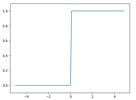
      

      

      Sigmoid Function

      import numpy as np
      import matplotlib.pylab as plt
      
      def sigmoid(x):
          return 1 / (1 + np.exp(-x))
      
      #  x = np.array([-1.0, 1.0, 2.0])
      #  print(y)
      
      x = np.arange(-5.0, 5.0, 0.1)
      y = sigmoid(x)
      
      plt.plot(x, y)
      plt.ylim(-0.1, 1.1)
      plt.show()
      

      

      %%Environment Setup !pip install numpy scipy matplotlib ipython scikit-learn pandas pillow Introduction to Artificial Neural Network Activation Function Step function import numpy as np import matplotlib.pylab as plt def step_function(x): return np.array(x>0, dtype=np.int) x = np.arange(-5.0, 5.0, 0.1) y = step_function(x) plt.plot(x, y) plt.ylim(-0.1, 1.1) plt.show() Sigmoid Function import numpy as np import matplotlib.pylab as plt def sigmoid(x): return 1 / (1 + np.exp(-x)) # x = np.array([-1.0, 1.0, 2.0]) # print(y) x = np.arange(-5.0, 5.0, 0.1) y = sigmoid(x) plt.plot(x, y) plt.ylim(-0.1, 1.1) plt.show() Relu Function $$ f(x)=max(0,x) $$ import numpy as np import matplotlib.pylab as plt def relu(x): return np.maximum(0, x) # x = np.array([-5.0, 5.0, 0.1]) # print(y) x = np.arange(-6.0, 6.0, 0.1) y = relu(x) plt.plot(x, y) plt.ylim(-1, 6) plt.show() 损失函数 平方和误差 Sum of squared error $$ E = \frac{1}{2} \sum_{k} (y_k -t_k)^2 $$ Cross Entropy error $$ E = - \sum_k t_k log\ y_k $$ References What is Rectified Linear Unit (ReLU)? | Introduction to ReLU Activation Function Machine Learning Glossary GitHub - NVIDIA-AI-IOT/deepstream_lpr_app: Sample app code for LPR deployment on DeepStream $$$ YOLO%%//milaiai.com:1313/post/yolo/%%2025-02-25%%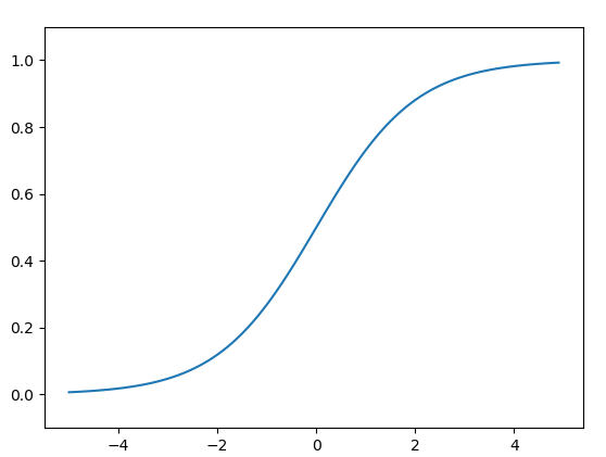

      onnx

      Introduction

      

      • ONNX官网：https://onnx.ai/

      • ONNX GitHub：https://github.com/onnx/onnx

      ONNX( Open Neural Network Exchange) 是 Facebook (现Meta) 和微软在2017年共同发布的，用于标准描述计算图的一种格式。ONNX通过定义一组与环境和平台无关的标准格式，使AI模型可以在不同框架和环境下交互使用，ONNX可以看作深度学习框架和部署端的桥梁，就像编译器的中间语言一样。由于各框架兼容性不一，我们通常只用 ONNX 表示更容易部署的静态图。硬件和软件厂商只需要基于ONNX标准优化模型性能，让所有兼容ONNX标准的框架受益。目前，ONNX主要关注在模型预测方面，使用不同框架训练的模型，转化为ONNX格式后，可以很容易的部署在兼容ONNX的运行环境中。目前，在微软，亚马逊 ，Facebook(现Meta) 和 IBM 等公司和众多开源贡献的共同维护下，ONNX 已经对接了下图的多种深度学习框架和多种推理引擎。

      %%onnx Introduction ONNX官网：https://onnx.ai/ ONNX GitHub：https://github.com/onnx/onnx ONNX( Open Neural Network Exchange) 是 Facebook (现Meta) 和微软在2017年共同发布的，用于标准描述计算图的一种格式。ONNX通过定义一组与环境和平台无关的标准格式，使AI模型可以在不同框架和环境下交互使用，ONNX可以看作深度学习框架和部署端的桥梁，就像编译器的中间语言一样。由于各框架兼容性不一，我们通常只用 ONNX 表示更容易部署的静态图。硬件和软件厂商只需要基于ONNX标准优化模型性能，让所有兼容ONNX标准的框架受益。目前，ONNX主要关注在模型预测方面，使用不同框架训练的模型，转化为ONNX格式后，可以很容易的部署在兼容ONNX的运行环境中。目前，在微软，亚马逊 ，Facebook(现Meta) 和 IBM 等公司和众多开源贡献的共同维护下，ONNX 已经对接了下图的多种深度学习框架和多种推理引擎。 ONNX Runtime 是由微软维护的一个跨平台机器学习推理加速器，它直接对接ONNX，可以直接读取.onnx文件并实现推理，不需要再把 .onnx 格式的文件转换成其他格式的文件。PyTorch借助ONNX Runtime也完成了部署的最后一公里，构建了 PyTorch –> ONNX –> ONNX Runtime 部署流水线，我们只需要将模型转换为 .onnx 文件，并在 ONNX Runtime 上运行模型即可。 Installation # 激活虚拟环境 conda activate env_name # env_name换成环境名称 # 安装onnx pip install onnx # 安装onnx runtime pip install onnxruntime # 使用CPU进行推理 # pip install onnxruntime-gpu # 使用GPU进行推理 ONNX模型的检验 import onnx # 我们可以使用异常处理的方法进行检验 try: # 当我们的模型不可用时，将会报出异常 onnx.checker.check_model(self.onnx_model) except onnx.checker.ValidationError as e: print("The model is invalid: %s"%e) else: # 模型可用时，将不会报出异常，并会输出“The model is valid!” print("The model is valid!") 模型转换为ONNX格式 import torch.onnx # 转换的onnx格式的名称，文件后缀需为.onnx onnx_file_name = "xxxxxx.onnx" # 我们需要转换的模型，将torch_model设置为自己的模型 model = torch_model # 加载权重，将model.pth转换为自己的模型权重 # 如果模型的权重是使用多卡训练出来，我们需要去除权重中多的module. 具体操作可以见5.4节 model = model.load_state_dict(torch.load("model.pth")) # 导出模型前，必须调用model.eval()或者model.train(False) model.eval() # dummy_input就是一个输入的实例，仅提供输入shape、type等信息 batch_size = 1 # 随机的取值，当设置dynamic_axes后影响不大 dummy_input = torch.randn(batch_size, 1, 224, 224, requires_grad=True) # 这组输入对应的模型输出 output = model(dummy_input) # 导出模型 torch.onnx.export(model, # 模型的名称 dummy_input, # 一组实例化输入 onnx_file_name, # 文件保存路径/名称 export_params=True, # 如果指定为True或默认, 参数也会被导出. 如果你要导出一个没训练过的就设为 False. opset_version=10, # ONNX 算子集的版本，当前已更新到15 do_constant_folding=True, # 是否执行常量折叠优化 input_names = ['input'], # 输入模型的张量的名称 output_names = ['output'], # 输出模型的张量的名称 # dynamic_axes将batch_size的维度指定为动态， # 后续进行推理的数据可以与导出的dummy_input的batch_size不同 dynamic_axes={'input' : {0 : 'batch_size'}, 'output' : {0 : 'batch_size'}}) 使用ONNX Runtime进行推理 # 导入onnxruntime import onnxruntime # 需要进行推理的onnx模型文件名称 onnx_file_name = "xxxxxx.onnx" # onnxruntime.InferenceSession用于获取一个 ONNX Runtime 推理器 ort_session = onnxruntime.InferenceSession(onnx_file_name) # 构建字典的输入数据，字典的key需要与我们构建onnx模型时的input_names相同 # 输入的input_img 也需要改变为ndarray格式 ort_inputs = {'input': input_img} # 我们更建议使用下面这种方法,因为避免了手动输入key # ort_inputs = {ort_session.get_inputs()[0].name:input_img} # run是进行模型的推理，第一个参数为输出张量名的列表，一般情况可以设置为None # 第二个参数为构建的输入值的字典 # 由于返回的结果被列表嵌套，因此我们需要进行[0]的索引 ort_output = ort_session.run(None,ort_inputs)[0] # output = {ort_session.get_outputs()[0].name} # ort_output = ort_session.run([output], ort_inputs)[0] PyTorch模型的输入为tensor，而ONNX的输入为array，因此我们需要对张量进行变换或者直接将数据读取为array格式，我们可以实现下面的方式进行张量到array的转化。 def to_numpy(tensor): return tensor.detach().cpu().numpy() if tensor.requires_grad else tensor.cpu().numpy() ONNX可视化 https://github.com/lutzroeder/netron 模型推理 如何使用torch.hub进行推理 依赖 pip install ultralytics -　使用 torch.hub.load( repo_or_dir, model, *args, ource='github', or 'local' force_reload=False, verbose=True, skip_validation=False, **kwargs) import torch model = torch.hub.load('ultralytics/yolov5', 'yolov5s') # official model model = torch.hub.load('ultralytics/yolov5:master', 'yolov5s') # from branch model = torch.hub.load('ultralytics/yolov5', 'custom', 'yolov5s.pt') # custom/local model model = torch.hub.load('.', 'custom', 'yolov5s.pt', source='local') # local repo 在线推理 import torch # Model loading # model = torch.hub.load("ultralytics/yolov5", "yolov5s") # Can be 'yolov5n' - 'yolov5x6', or 'custom' model = torch.hub.load( "./", "custom", path=f"{local_model_path}/{model_name}", device=device, source='local', force_reload=[True if "refresh_yolov5" in opt else False][0], _verbose=True, ) # Inference on images img = "https://ultralytics.com/images/zidane.jpg" # Can be a file, Path, PIL, OpenCV, numpy, or list of images # Run inference results = model(img) # Display results results.print() # Other options: .show(), .save(), .crop(), .pandas(), etc. 评论 1. 需要安装ultralytics与torchvision, 可能不太适合Raspery Pi等嵌入式平台 2. 需要yolo源码，需要hubconf.py入口脚本 3. model = torch.hub.load("ultralytics/yolov5", "yolov5s")是从github下载 Jetson Nano version nvcc $ nvcc --version nvcc: NVIDIA (R) Cuda compiler driver Copyright (c) 2005-2024 NVIDIA Corporation Built on Wed_Aug_14_10:14:07_PDT_2024 Cuda compilation tools, release 12.6, V12.6.68 Build cuda_12.6.r12.6/compiler.34714021_0 References 9.1 使用ONNX进行部署并推理 — 深入浅出PyTorch) Errors Start Jupyter Notebook inside vscde Q: The kernel failed to start due to the missing module 'decorator'. Consider installing this module. Click <a href='https://aka.ms/kernelFailuresMissingModule'>here</a> for more info. A: conda install --name yolo --update-deps --force-reinstall ipykernel OpenCV CUDA Q: When use model = cv2.dnn.readNetFromONNX('../runs/train/exp3/weights/best.onnx') model.setPreferableBackend(cv2.dnn.DNN_BACKEND_CUDA) # cv::dnn::DNN_BACKEND_CUDA. DNN_BACKEND_OPENCV model.setPreferableTarget(cv2.dnn.DNN_TARGET_CUDA) # DNN_TARGET_CPU Get this error: Traceback (most recent call last): File "/home/nvidia/yolov5/detect/./cv_onnx.py", line 40, in <module> outputs = model.forward() cv2.error: OpenCV(4.11.0) /io/opencv/modules/dnn/src/net_impl.cpp:119: error: (-215:Assertion failed) preferableBackend != DNN_BAC KEND_CUDA || IS_DNN_CUDA_TARGET(preferableTarget) in function 'validateBackendAndTarget' $$$ Pytorch with CUDA%%//milaiai.com:1313/post/python/%%2025-01-20%%

      Introduction

      • pytorch -> C++ -> CUDA
      • pybind: call C++ from python
      • CUDA GPU architechture

      

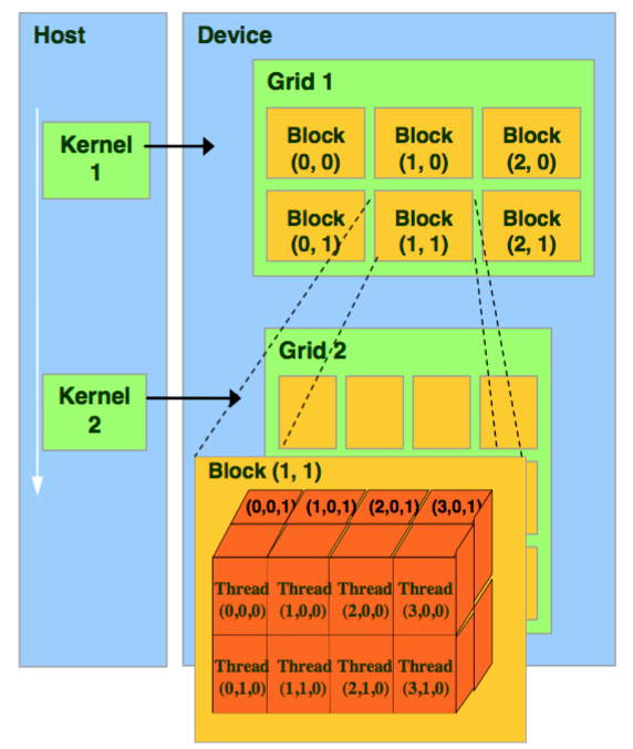
      • CUDA: grid -> block->thread
      • 为什么要有block这个中间层?
        • block 上限： $(2^{31}-1)*2^{16}*2^{16}$
        • Thread上限: 1024

      Conda

      • https://docs.anaconda.com/free/anaconda/install/linux/

        wget -c https://repo.anaconda.com/archive/Anaconda3-2023.09-0-Linux-x86_64.sh
        

      pip

      • pip使用国内镜像源

      • Usefusl

        pip3 install numpy -i https://pypi.tuna.tsinghua.edu.cn/simple
        

      • ~/.pip/pip.conf

        [global]
        index-url = https://pypi.tuna.tsinghua.edu.cn/simple
        [install]
        trusted-host = https://pypi.tuna.tsinghua.edu.cn
        

      • pip国内的一些镜像

        %%Introduction pytorch -> C++ -> CUDA pybind: call C++ from python CUDA GPU architechture CUDA: grid -> block->thread 为什么要有block这个中间层? block 上限： $(2^{31}-1)*2^{16}*2^{16}$ Thread上限: 1024 Conda https://docs.anaconda.com/free/anaconda/install/linux/ wget -c https://repo.anaconda.com/archive/Anaconda3-2023.09-0-Linux-x86_64.sh pip pip使用国内镜像源 Usefusl pip3 install numpy -i https://pypi.tuna.tsinghua.edu.cn/simple ~/.pip/pip.conf [global] index-url = https://pypi.tuna.tsinghua.edu.cn/simple [install] trusted-host = https://pypi.tuna.tsinghua.edu.cn pip国内的一些镜像 阿里云 http://mirrors.aliyun.com/pypi/simple/ 中国科技大学 https://pypi.mirrors.ustc.edu.cn/simple/ 豆瓣(douban) http://pypi.douban.com/simple/ 清华大学 https://pypi.tuna.tsinghua.edu.cn/simple/ 中国科学技术大学 http://pypi.mirrors.ustc.edu.cn/simple/ Pytorch https://pytorch.org/ pip3 install torch torchvision torchaudio Pip source list https://www.cnblogs.com/chenjo/p/14071864.html ~/.pip/pip.conf [global] index-url = https://pypi.tuna.tsinghua.edu.cn/simple [install] trusted-host=mirrors.aliyun.com Set source list for pip install pip install pymysql -i https://pypi.tuna.tsinghua.edu.cn/simple/ // 国内源 pip install 包名-i http://pypi.douban.com/simple/ --trusted-host pypi.douban.com Environment Building conda create -n cppcuda python=3.8 conda activate cppcuda Install pytorch python -m pip install pip -U pip3 install torch torchvision torchaudio pytorch path how to check path import torch print(torch.__file__) path example: "/usr/include/python3.8", "/home/.local/lib/python3.8/site-packages/torch/include/", "/home/.local/lib/python3.8/site-packages/torch/include/torch/csrc/api/include" Python setup Example for CppExtension from setuptools import setup from torch.utils.cpp_extension import BuildExtension, CppExtension setup( name='cppcuda_tutorial', version='1.0', author='qingbao', author_email='<EMAIL>', description='cppcuda example', long_description='A tutorial for using C++ and CUDA in PyTorch', long_description_content_type='text/markdown', ext_modules=[ CppExtension( name='cppcuda_tutorial', sources=['interplation.cpp']), ], cmdclass={ 'build_ext': BuildExtension}, ) General use case non parallel computation, e.g. volume rendering lots of sequential computation Example: linear interpolation Bilinear interpolation Trilinear interpolation Input feats: (N, 8, F) N: 多少个volume 8： 8个顶点 F: 每个顶点的特征 Output points: (N, 3) 差值后的点 平行运算： N个点 F平行 如何计算block大小 const int N = feats.size(0); const int F = feats.size(2); // torch::zeros({N, F}, torch::dtype(torch::kInt32).device(feats.device())); torch::Tensor feat_interp = torch::zeros({N, F}, feats.options()); const dim3 threads(16, 16); // max threads:256, two dimension, each use 16 threads const blocks((N + threads.x -1)/threads.x, (F + threads.y -1)/threads.y); Issues unsupported clang version /usr/local/cuda/bin/../targets/x86_64-linux/include/crt/host_config.h:151:2: [cmake] error: -- unsupported clang version! clang version must be less than 16 and [cmake] greater than 3.2 . The nvcc flag '-allow-unsupported-compiler' can be used [cmake] to override this version check; however, using an unsupported host compiler [cmake] may cause compilation failure or incorrect run time execution. Use at your [cmake] own risk. [cmake] [cmake] 151 | #error -- unsupported clang version! clang version must be less than 16 and greater than 3.2 . The nvcc flag '-allow-unsupported-compiler' can be used to override this version check; however, using an unsupported host compiler may cause compilation failure or incorrect run time execution. Use at your own risk. [cmake] | ^ [cmake] [cmake] 1 error generated. Solution: Use clang less than 16. set(CMAKE_C_COMPILER /usr/bin/clang-13) set(CMAKE_CXX_COMPILER /usr/bin/clang++-13) Failed to initialize NumPy .local/lib/python3.8/site-packages/torch/nn/modules/transformer.py:20: UserWarning: Failed to initialize NumPy: numpy.core.multiarray failed to import (Triggered internally at ../torch/csrc/utils/tensor_numpy.cpp:84.) device: torch.device = torch.device(torch._C._get_default_device()), # torch.device('cpu'), Solution: python -m pip install pip -U setuptools _check_cuda_version(compiler_name, compiler_version) File "/home/qingbao/.local/lib/python3.8/site-packages/torch/utils/cpp_extension.py", line 411, in _check_cuda_version raise ValueError("setuptools>=49.4.0 is required") ValueError: setuptools>=49.4.0 is required QT PySide6 PySide6 pip install PySide6 --trusted-host mirrors.aliyun.com Vscode PySide plugin PYQT Integration Path whereis pyside6-lupdate whereis pyside6-designer whereis pyside6-qmlls whereis pyside6-qml whereis pyside6-qmlformat pyside6-uic pyside6-rcc Run pyside6-designer References Pytorch+cpp/cuda extension 教學 tutorial 1 https://docs.nvidia.com/cuda/cuda-c-programming-guide/index.html#features-and-technical-specifications__technical-specifications-per-compute-capability https://github.com/kwea123/pytorch-cppcuda-tutorial pip安装包报错Could not find a version that satisfies the requirement pymysql (from versions: none) $$$ ORB_SLAM3%%//milaiai.com:1313/post/orb-slam/%%2024-12-10%%

        Get ORB_SLAM3

        git clone https://github.com/yubaoliu/ORB_SLAM3.git
        cd ORB_SLAM3
        git checkout dev
        

        Deploy ORB_SLAM3

        • Build OpenCV OpenCV will be installed when you install the ROS.

        • Build thirdparties

        chmod +x build.sh
        ./build.sh
        

        使用Realsense运行ORB_SLAM3

        • Start realsense camera node

        roslaunch realsense2_camera rs_rgbd.launch
        

        • Start ORB_SLAM3 node

        roslaunch orb_slam3 realsense.launch 
        

        %%Get ORB_SLAM3 git clone https://github.com/yubaoliu/ORB_SLAM3.git cd ORB_SLAM3 git checkout dev Deploy ORB_SLAM3 Build OpenCV OpenCV will be installed when you install the ROS. Build thirdparties chmod +x build.sh ./build.sh 使用Realsense运行ORB_SLAM3 Start realsense camera node roslaunch realsense2_camera rs_rgbd.launch Start ORB_SLAM3 node roslaunch orb_slam3 realsense.launch $$$ SLAM%%//milaiai.com:1313/post/slam/%%2024-12-10%%

        研究机构

        美国卡耐基梅陇大学机器人研究所

        研究所主页：https://www.ri.cmu.edu/

        发表论文：https://www.ri.cmu.edu/pubs/

        %%研究机构 美国卡耐基梅陇大学机器人研究所 研究所主页：https://www.ri.cmu.edu/ 发表论文：https://www.ri.cmu.edu/pubs/ 优秀团队成员：Michael Kaess、Sebastian Scherer 研究方向：机器人感知、结构，服务型、运输、制造业、现场机器等 美国加州大学圣地亚哥分校语境机器人研究所 实验室主页：https://existentialrobotics.org/index.html 发表论文汇总：https://existentialrobotics.org/pages/publications.html 优秀团队成员：Nikolay Atanasov 研究方向：多模态环境理解，语义导航，自主信息获取 美国特拉华大学机器人感知与导航组 实验室主页：https://sites.udel.edu/robot/ 发表论文汇总：https://sites.udel.edu/robot/publications/ Github 地址：https://github.com/rpng?page=2 优秀团队成员：黄国权教授、左星星等 研究方向：SLAM、VINS、语义定位与建图等 美国麻省理工学院航空航天实验室 实验室主页：http://acl.mit.edu/ 发表论文：http://acl.mit.edu/publications 优秀团队成员：Jonathan P. How 教授、Kasra Khosoussi（SLAM 图优化） 研究方向：位姿估计与导航，路径规划，控制与决策，机器学习与强化学习 美国麻省理工学院 SPARK 实验室 实验室主页：http://web.mit.edu/sparklab/ 优秀团队成员：Luca Carlone 教授 研究方向：移动机器人环境感知 美国麻省理工学院海洋机器人组 实验室主页：https://marinerobotics.mit.edu/ （隶属于 MIT 计算机科学与人工智能实验室） 发表论文汇总：https://marinerobotics.mit.edu/biblio 优秀团队成员：John Leonard 教授 研究方向：水下或陆地移动机器人导航与建图 美国明尼苏达大学多元自主机器人系统实验室 实验室主页：http://mars.cs.umn.edu/index.php 发表论文汇总：http://mars.cs.umn.edu/publications.php VIO 相关研究：http://mars.cs.umn.edu/research/vins_overview.php 优秀团队成员：Stergios I. Roumeliotis 研究方向：视觉、激光、惯性导航系统，移动设备大规模三维建模与定位 美国宾夕法尼亚大学 Vijay Kumar 实验室 实验室主页：https://www.kumarrobotics.org/ 发表论文：https://www.kumarrobotics.org/publications/ 研究成果视频：https://www.youtube.com/user/KumarLabPenn/videos 研究方向：自主微型无人机 加拿大蒙特利尔大学 机器人与嵌入式 AI 实验室 实验室主页：http://montrealrobotics.ca/ 优秀团队成员：Liam Paull 教授 研究方向：SLAM，不确定性建模 加拿大舍布鲁克大学智能、交互、综合、跨学科机器人实验室 实验室主页：https://introlab.3it.usherbrooke.ca/ 项目主页：http://introlab.github.io/rtabmap/ 研究方向：移动机器人软硬件设计 瑞士苏黎世大学机器人与感知课题组 实验室主页：http://rpg.ifi.uzh.ch/index.html 发表论文汇总：http://rpg.ifi.uzh.ch/publications.html Github 代码公开地址：https://github.com/uzh-rpg 事件相机项目主页：http://rpg.ifi.uzh.ch/research_dvs.html 优秀团队成员：Davide Scaramuzza 研究方向：移动机器人、无人机环境感知与导航，VISLAM，事件相机 瑞士苏黎世联邦理工计算机视觉与几何实验室 实验室主页：http://www.cvg.ethz.ch/index.php 发表论文：http://www.cvg.ethz.ch/publications/ 优秀团队成员：Marc Pollefeys、Johannes L. Schönberger 研究方向：定位、三维重建、语义分割、机器人视觉 英国帝国理工学院戴森机器人实验室 实验室主页：https://www.imperial.ac.uk/dyson-robotics-lab/ 发表论文：https://www.imperial.ac.uk/dyson-robotics-lab/publications/ 开源代码：MonoSLAM、CodeSLAM、ElasticFusion、KinectFusion 优秀团队成员：Andrew Davison 研究方向：机器人视觉场景与物体理解、机器人操纵 英国牛津大学信息工程学 实验室主页：http://www.robots.ox.ac.uk/ 主动视觉实验室：http://www.robots.ox.ac.uk/ActiveVision/ 牛津机器人学院：https://ori.ox.ac.uk/ 发表论文汇总： 主动视觉实验室：http://www.robots.ox.ac.uk/ActiveVision/Publications/index.html 机器人学院：https://ori.ox.ac.uk/publications/papers/ 优秀团队成员：David Murray Maurice Fallon 研究方向：SLAM、目标跟踪、运动结构、场景增强、移动机器人运动规划、导航与建图等等等 德国慕尼黑工业大学计算机视觉组 实验室主页：https://vision.in.tum.de/research/vslam 发表论文汇总：https://vision.in.tum.de/publications 代表作：DSO、LDSO、LSD_SLAM、DVO_SLAM Github 地址：https://github.com/tum-vision 优秀团队成员：Daniel Cremers、Jakob Engel 研究方向：三维重建、机器人视觉、深度学习、视觉 SLAM 等 德国弗莱堡大学智能自主系统实验室 实验室主页：http://ais.informatik.uni-freiburg.de/index_en.php 发表论文汇总：http://ais.informatik.uni-freiburg.de/publications/index_en.php 开放数据集：http://aisdatasets.informatik.uni-freiburg.de/ 优秀团队成员：Wolfram Burgard 研究方向：多机器人导航与协作，环境建模与状态估计 西班牙萨拉戈萨大学机器人、感知与实时组 SLAM 实验室 实验室主页：http://robots.unizar.es/slamlab/ 发表论文：http://robots.unizar.es/slamlab/?extra=3 优秀团队成员：J. M. M. Montiel 研究方向：视觉 SLAM、物体 SLAM、非刚性 SLAM、机器人、增强现实 西班牙马拉加大学机器感知与智能机器人课题组 实验室主页：http://mapir.uma.es/mapirwebsite/index.php/topics-2.html 发表论文汇总：http://mapir.isa.uma.es/mapirwebsite/index.php/publications-menu-home.html 优秀团队成员：Francisco-Angel Moreno、Ruben Gomez-Ojeda 研究方向：自主机器人、人工嗅觉、计算机视觉 奥地利格拉茨技术大学计算机图形学与视觉研究所 实验室主页：https://www.tugraz.at/institutes/icg/home/ 优秀团队成员：Dieter Schmalstieg教授、Friedrich Fraundorfer 教授 研究方向：AR/VR，机器人视觉，机器学习，目标识别与三维重建 波兰波兹南工业大学移动机器人实验室 实验室主页：http://lrm.put.poznan.pl/ Github 主页：https://github.com/LRMPUT 研究方向：SLAM，机器人运动规划，控制 澳大利亚机器人视觉中心 实验室主页：https://www.roboticvision.org/ 人物：https://www.roboticvision.org/rv_person_category/researchers/ 发表论文汇总：https://www.roboticvision.org/publications/scientific-publications/ 优秀团队成员：Yasir Latif、Ian D Reid 研究方向：AR/VR，机器人视觉，机器学习，目标识别与三维重建 日本国立先进工业科学技术研究所 人工智能研究中心：https://www.airc.aist.go.jp/en/intro/ 优秀团队成员：Ken Sakurada、Shuji Oishi 香港科技大学空中机器人实验室 实验室主页：http://uav.ust.hk/ 发表论文：http://uav.ust.hk/publications/ 代码公开地址：https://github.com/HKUST-Aerial-Robotics 优秀团队成员：沈邵劼教授 研究方向：空中机器人在复杂环境下的自主运行，包括状态估计、建图、运动规划、多机器人协同以及低成本传感器和计算组件的实验平台开发。 香港科技大学机器人与多感知实验室 RAM-LAB 实验室主页：https://www.ram-lab.com/ 发表论文：https://www.ram-lab.com/publication/ 优秀团队成员：刘明教授 研究方向：无人车；无人船；室内定位；机器学习。 香港中文大学天石机器人实验室 实验室主页：http://ri.cuhk.edu.hk/ 优秀团队成员：刘云辉教授、李浩昂 研究方向：工业、物流、手术机器人，三维影像，机器学习 浙江大学 CAD&CG 国家重点实验室 实验室主页：http://www.zjucvg.net/ Github 代码地址：https://github.com/zju3dv 优秀团队成员：章国峰教授 研究方向：SFM/SLAM，三维重建，增强现实 2.SLAMer 邹丹平（上海交通大学） 研究方向：视觉 SLAM，SFM，多源导航，微型无人机 个人主页：http://drone.sjtu.edu.cn/dpzou/index.php Co-SLAM：Zou D, Tan P. Coslam: Collaborative visual slam in dynamic environments[J]. IEEE transactions on pattern analysis and machine intelligence, 2012, 35(2): 354-366.（代码：https://github.com/danping/CoSLAM ） StructSLAM：Zhou H, Zou D, Pei L, et al. StructSLAM: Visual SLAM with building structure lines[J]. IEEE Transactions on Vehicular Technology, 2015, 64(4): 1364-1375.（项目主页：http://drone.sjtu.edu.cn/dpzou/project/structslam.php ） StructVIO：Zou D, Wu Y, Pei L, et al. StructVIO: visual-inertial odometry with structural regularity of man-made environments[J]. IEEE Transactions on Robotics, 2019, 35(4): 999-1013. 布树辉教授（西北工业大学智能系统实验室） 研究方向：语义定位与建图、SLAM、在线学习与增量学习 个人主页：http://www.adv-ci.com/blog/ 布老师的课件：http://www.adv-ci.com/blog/course/ 实验室 2018 年暑期培训资料：https://github.com/zdzhaoyong/SummerCamp201 Alejo Concha（Oculus VR，西班牙萨拉戈萨大学） 研究方向：SLAM，单目稠密重建，传感器融合 个人主页：https://sites.google.com/view/alejoconcha/ Github：https://github.com/alejocb IROS 2015 单目平面重建：DPPTAM: Dense piecewise planar tracking and mapping from a monocular sequence （代码:https://github.com/alejocb/dpptam ） IROS 2017 开源 RGB-D SLAM：RGBDTAM: A Cost-Effective and Accurate RGB-D Tracking and Mapping System（代码：https://github.com/alejocb/rgbdtam ） Srikumar Ramalingam（美国犹他大学计算机学院） 研究方向：三维重构、语义分割、视觉 SLAM、图像定位、深度神经网络 2D-3D 定位：Ataer-Cansizoglu E, Taguchi Y, Ramalingam S. Pinpoint SLAM: A hybrid of 2D and 3D simultaneous localization and mapping for RGB-D sensors[C]//2016 IEEE international conference on robotics and automation (ICRA). IEEE, 2016: 1300-1307 Frank Dellaert（美国佐治亚理工学院机器人与智能机器研究中心） 研究方向：SLAM，图像时空重构 Choudhary S, Trevor A J B, Christensen H I, et al. SLAM with object discovery, modeling and mapping[C]//2014 IEEE/RSJ International Conference on Intelligent Robots and Systems. IEEE, 2014: 1018-1025. Alexander Vakhitov（三星莫斯科 AI 中心） 研究方向：SLAM，几何视觉 个人主页：https://alexandervakhitov.github.io/ 点线定位：Pumarola A, Vakhitov A, Agudo A, et al. Relative localization for aerial manipulation with PL-SLAM[M]//Aerial Robotic Manipulation. Springer, Cham, 2019: 239-248. 学习型线段：IEEE Access 2019 Learnable line segment descriptor for visual SLAM（代码：https://github.com/alexandervakhitov/lld-slam ） Papers MetaSLAM MetaSLAM BioSLAM [1] P. Yin, A. Abuduweili, S. Zhao, C. Liu, and S. Scherer, BioSLAM: A Bio-inspired Lifelong Memory System for General Place Recognition, Aug. 30, 2022, arXiv: arXiv:2208.14543. https://metaslam.github.io/ $$$ AGV机器人导航%%//milaiai.com:1313/post/agv/%%2024-08-31%%

        Comany

        • 北京视频案例-途灵机器人

        https://www.a-g-v.com/uploads/video/20230704/1688440958215838.mp4

        思岚

        • https://www.slamware.com/Docs/QuickStart
        • Support ROS
        • https://slam.cgabc.xyz/zh-cn/latest/
        • https://github.com/Slamtec/slamkit_ros
        • https://www.slamware.com/

        万集

        BluRobotics

        ANT

        镭神智能

        • https://www.leishen-lidar.com/

        深圳市智人科技有限公司

        -　http://www.wittyrobotics.com/

        科钛

        • http://www.cotek-robotics.com/yyal

        眸视科技

        • https://www.mskjrobot.com/

        Localization

        激光三角定位

        

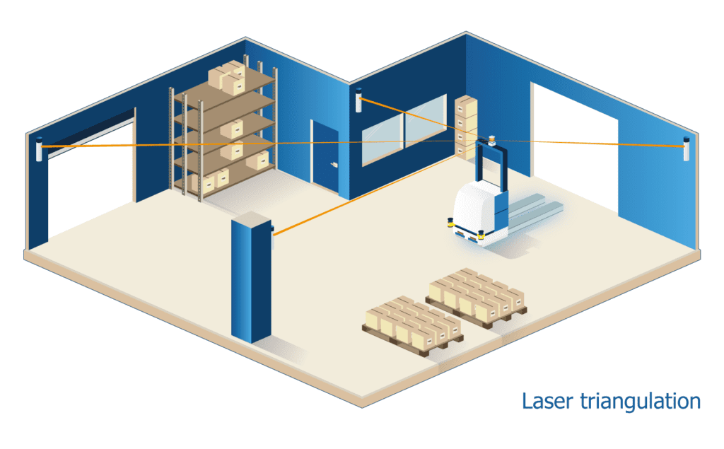
        References

        • 十种主流的AGV导航方式，你知道几种？–机器视觉网

        • AGV导航方法2：虚拟路径跟随

        • 基于二维码视觉导航的AGV自动充电方案

        %%Comany 北京视频案例-途灵机器人 https://www.a-g-v.com/uploads/video/20230704/1688440958215838.mp4 思岚 https://www.slamware.com/Docs/QuickStart Support ROS https://slam.cgabc.xyz/zh-cn/latest/ https://github.com/Slamtec/slamkit_ros https://www.slamware.com/ 万集 BluRobotics ANT 镭神智能 https://www.leishen-lidar.com/ 深圳市智人科技有限公司 -　http://www.wittyrobotics.com/ 科钛 http://www.cotek-robotics.com/yyal 眸视科技 https://www.mskjrobot.com/ Localization 激光三角定位 References 十种主流的AGV导航方式，你知道几种？–机器视觉网 AGV导航方法2：虚拟路径跟随 基于二维码视觉导航的AGV自动充电方案 $$$ DALL-E%%//milaiai.com:1313/post/dall-e/%%2024-08-31%%

        2021 DALL-E

        [1] A. Ramesh et al., Zero-Shot Text-to-Image Generation, Feb. 26, 2021, arXiv: arXiv:2102.12092.

        • https://openai.com/index/dall-e/

        • https://github.com/openai/DALL-E

        • https://www.dall-efree.com/

        • VQGAN, VAE

        • codebook 定义好所有已知的特征

        

        

        

        %%2021 DALL-E [1] A. Ramesh et al., Zero-Shot Text-to-Image Generation, Feb. 26, 2021, arXiv: arXiv:2102.12092. https://openai.com/index/dall-e/ https://github.com/openai/DALL-E https://www.dall-efree.com/ VQGAN, VAE codebook 定义好所有已知的特征 $$$ LangChain%%//milaiai.com:1313/post/langchain/%%2024-08-31%%

        Introduction

        Build context-aware reasoning applications

        LangChain is a framework for developing applications powered by large language models (LLMs).

        • https://python.langchain.com/v0.2/docs/introduction/

        

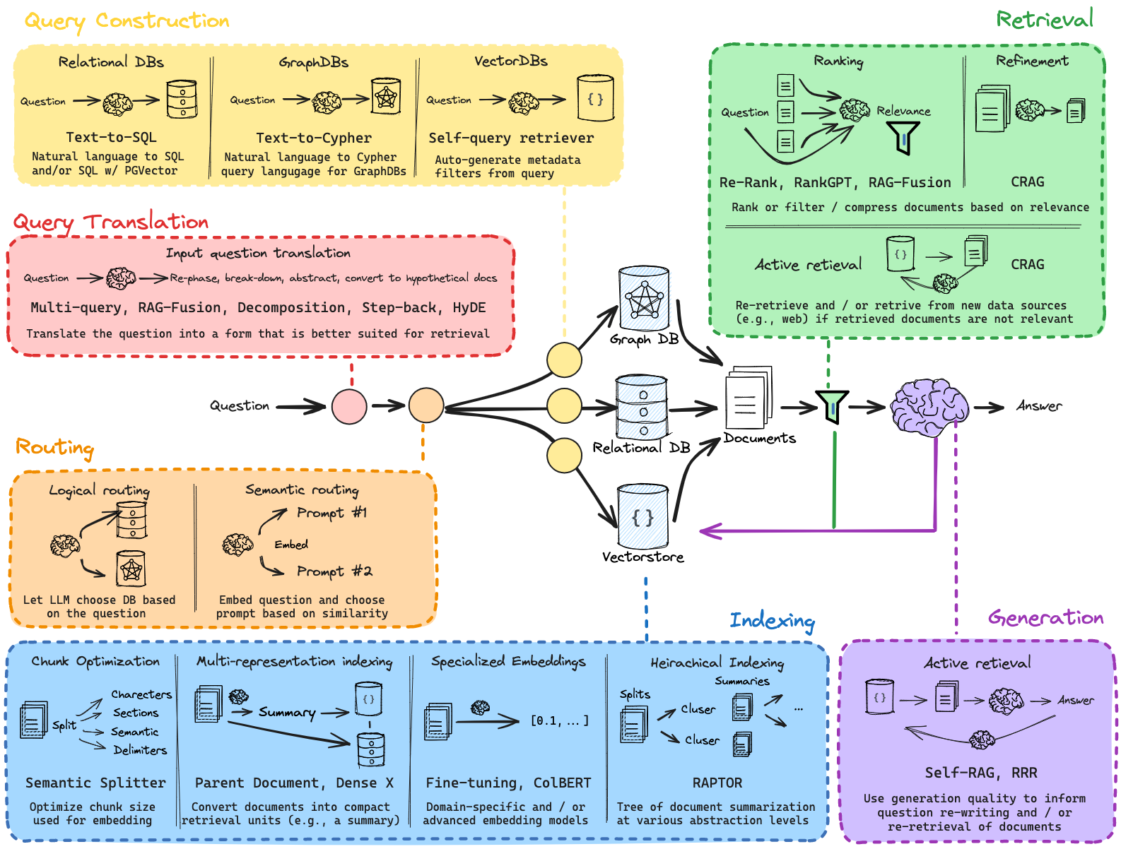
        User Guide

        Install

        pip install langchain
        
        #--optional--
        pip install langchain_community langchain_ollama langchain_chroma
        

        Use Ollama

        有两种方式使用ollama本地大模型

        • Method: use langchain_community

        # Method 1: Using LangChain's base classes and components directly
        from langchain_community.llms import Ollama
        from langchain_core.prompts import ChatPromptTemplate
        from langchain_core.output_parsers import StrOutputParser
        
        output_parser = StrOutputParser()
        
        llm = Ollama(model="llama3.1")
        prompt = ChatPromptTemplate.from_messages([
            ("system", "You are world class technical documentation writer."),
            ("user", "{input}")
        ])
        chain = prompt | llm | output_parser
        
        print(chain.invoke({"input": "how can langsmith help with testing?"}))
        

        • Method: use langchain_ollama

        # Method 2: Using LangChain's Ollama wrapper
        from langchain_ollama import OllamaLLM
        
        model = OllamaLLM(model="llama3.1")
        res = model.invoke("Come up with 10 names for a song about parrots")
        print(res)
        

        References

        • https://github.com/XingYu-Zhong/LangChainStudy

          %%Introduction Build context-aware reasoning applications LangChain is a framework for developing applications powered by large language models (LLMs). https://python.langchain.com/v0.2/docs/introduction/ User Guide Install pip install langchain #--optional-- pip install langchain_community langchain_ollama langchain_chroma Use Ollama 有两种方式使用ollama本地大模型 Method: use langchain_community # Method 1: Using LangChain's base classes and components directly from langchain_community.llms import Ollama from langchain_core.prompts import ChatPromptTemplate from langchain_core.output_parsers import StrOutputParser output_parser = StrOutputParser() llm = Ollama(model="llama3.1") prompt = ChatPromptTemplate.from_messages([ ("system", "You are world class technical documentation writer."), ("user", "{input}") ]) chain = prompt | llm | output_parser print(chain.invoke({"input": "how can langsmith help with testing?"})) Method: use langchain_ollama # Method 2: Using LangChain's Ollama wrapper from langchain_ollama import OllamaLLM model = OllamaLLM(model="llama3.1") res = model.invoke("Come up with 10 names for a song about parrots") print(res) References https://github.com/XingYu-Zhong/LangChainStudy https://www.langchain.com/ https://chat.langchain.com/ LangChain｜Ollama结合LangChain使用的速通版 https://www.llamaindex.ai/ Langchain最新0.2版讲解 $$$ 银行卡开户%%//milaiai.com:1313/post/bank/%%2024-05-08%%

          香港银行卡开户

          实体银行

          大家好,今天给大家分享一下我在香港开户的经历. 我是今年5月1号劳动节前去的香港. 我在去之前也看了几个相关视频,做了些准备工作.但是去了香港之后才发现,真实情况与那些视频里介绍的还是有很大不同的.今天跟大家分享一下我的开户经历.

          %%香港银行卡开户 实体银行 大家好,今天给大家分享一下我在香港开户的经历. 我是今年5月1号劳动节前去的香港. 我在去之前也看了几个相关视频,做了些准备工作.但是去了香港之后才发现,真实情况与那些视频里介绍的还是有很大不同的.今天跟大家分享一下我的开户经历. 先介绍一下实体银行,我这里分了三列.第一列是我申请成功的,是不需要预约的,每家银行直接去银行,半天左右的时间可以办完. 不过银行里开户的人可以会很多,大部分时间可能都是在排队.建议大家能预约的话,尽量提前预约一下. 汇丰是最好申请的,只需要提供港澳通行证及入境小票.开完户,存几百元就行了. 恒生银行之前是不给大陆客户开户的,近期才允许大陆客户开户的.恒生银行开户要谨慎很多.要看你三个月以内的地址证明,收入明细等等. 中国银行(香港)开户要注意的是,要提供纸质版的地址证明. 我去的时候只带了电子版的,没有带纸质版的,银行让我去打印社(快图美)打印了一份.香港打印费是很贵的,打印一张彩色的需要8元. 开户完如果存款1万的话,可以当场拿卡. 不然的话,存一千元,卡片会邮寄给你.中国银行每笔国内汇款入帐都要收取手续费. 第二列中字头的银行都是需要事先预约的.我去的时候工行亚洲预约都已经预约到7月份了.如果大家要开中字头的银行的话,建议大家提前一个月预约. 中信国际有的网点不预约也行,我去的那家中信银行,让我必须买保险才能办理开户.保险是5年的封闭期,年利率5.3%, 我没有办理. 第三列的花旗银行,这个适合高端人群,如果你有150万的话,可以选择开这个.没有的话可能也能开,不过可能有些条件. 比如说每年有管理费之类的. 开户材料 开户材料都是比较好准备的. 地址证明要精确到门牌号. 可以使用信用卡账单. 如果申请中字头银行,最好事先打印下来. 现金建议带1万人民币,不用换成港元. 有些银行需要提供资金证明,资金证明可以是工资流水,国内或国外证券账户. 如果申请恒生银行的话,可能需要提供10万以上的存款证明或者证券账户. 开户地址可以选在尖沙咀附近,这里遍地都是银行,而且这附近有不少比较便宜的旅店. 如果你打算当天就离港,不住宿的话,你可以在太和地铁站附近开户. 太和距离罗湖口岸很近. 虚拟银行 这几家虚拟银行, 蚂蚁银行, 众安银行, 天星银行, 理慧銀行, 富融銀行. 开户都很简单,只要你人在香港就能开户. 你可以在手机应用商城,例如Google Play里下载应APP. 全程手机上开通. 大家可以在排队开户的时候顺便把他们开了. 谢谢大家的收看,以上内容仅供参考. 参考材料 恒生银行开户材料 $$$ Dataset%%//milaiai.com:1313/post/dataset/%%2024-05-06%%

          网上找到的国内下载地址

          Refer: https://blog.csdn.net/qq_36170626/article/details/94902166

          • TUM

          链接：https://pan.baidu.com/s/1nwXtGqH 密码：lsgr

          • KITTI

          链接：https://pan.baidu.com/s/1htFmXDE 密码：uu20

          %%网上找到的国内下载地址 Refer: https://blog.csdn.net/qq_36170626/article/details/94902166 TUM 链接：https://pan.baidu.com/s/1nwXtGqH 密码：lsgr KITTI 链接：https://pan.baidu.com/s/1htFmXDE 密码：uu20 KITTI gt 链接:https://pan.baidu.com/s/1lX6VEhl2pPpU_3Wcp3VYdg 提取码:5ux2 DSO 链接：https://pan.baidu.com/s/1eSRmeZK 密码：6x5b Mono 链接：https://pan.baidu.com/s/1jKaNB3C 密码：u57r EuRoC 链接：https://pan.baidu.com/s/1miXf40o 密码：xm59 KITTI raw data:https://pan.baidu.com/s/1TyXbifoTHubu3zt4jZ90Wg 提取码: n9ys EuRoC EuRoC_download # Machine Hall http://robotics.ethz.ch/~asl-datasets/ijrr_euroc_mav_dataset/machine_hall/MH_01_easy/MH_01_easy.zip http://robotics.ethz.ch/~asl-datasets/ijrr_euroc_mav_dataset/machine_hall/MH_02_easy/MH_02_easy.zip http://robotics.ethz.ch/~asl-datasets/ijrr_euroc_mav_dataset/machine_hall/MH_03_medium/MH_03_medium.zip http://robotics.ethz.ch/~asl-datasets/ijrr_euroc_mav_dataset/machine_hall/MH_04_difficult/MH_04_difficult.zip http://robotics.ethz.ch/~asl-datasets/ijrr_euroc_mav_dataset/machine_hall/MH_05_difficult/MH_05_difficult.zip http://robotics.ethz.ch/~asl-datasets/ijrr_euroc_mav_dataset/machine_hall/MH_01_easy/MH_01_easy.bag http://robotics.ethz.ch/~asl-datasets/ijrr_euroc_mav_dataset/machine_hall/MH_02_easy/MH_02_easy.bag http://robotics.ethz.ch/~asl-datasets/ijrr_euroc_mav_dataset/machine_hall/MH_03_medium/MH_03_medium.bag http://robotics.ethz.ch/~asl-datasets/ijrr_euroc_mav_dataset/machine_hall/MH_04_difficult/MH_04_difficult.bag http://robotics.ethz.ch/~asl-datasets/ijrr_euroc_mav_dataset/machine_hall/MH_05_difficult/MH_05_difficult.bag # Vicon Room 1 http://robotics.ethz.ch/~asl-datasets/ijrr_euroc_mav_dataset/vicon_room1/V1_01_easy/V1_01_easy.zip http://robotics.ethz.ch/~asl-datasets/ijrr_euroc_mav_dataset/vicon_room1/V1_02_medium/V1_02_medium.zip http://robotics.ethz.ch/~asl-datasets/ijrr_euroc_mav_dataset/vicon_room1/V1_03_difficult/V1_03_difficult.zip # Vicon Room 2 http://robotics.ethz.ch/~asl-datasets/ijrr_euroc_mav_dataset/vicon_room2/V2_01_easy/V2_01_easy.zip http://robotics.ethz.ch/~asl-datasets/ijrr_euroc_mav_dataset/vicon_room2/V2_02_medium/V2_02_medium.zip http://robotics.ethz.ch/~asl-datasets/ijrr_euroc_mav_dataset/vicon_room2/V2_03_difficult/V2_03_difficult.zip # Calibration Dataset http://robotics.ethz.ch/~asl-datasets/ijrr_euroc_mav_dataset/calibration_datasets/ Loop closure New College and City Centre https://www.robots.ox.ac.uk/~mobile/IJRR_2008_Dataset/data.html Papers DexCap [1] C. Wang, H. Shi, W. Wang, R. Zhang, L. Fei-Fei, and C. K. Liu, DexCap: Scalable and Portable Mocap Data Collection System for Dexterous Manipulation, Jul. 04, 2024, arXiv: arXiv:2403.07788. Universal Manipulation Interface [1] C. Chi et al., Universal Manipulation Interface: In-The-Wild Robot Teaching Without In-The-Wild Robots, Mar. 05, 2024, arXiv: arXiv:2402.10329. HIRO Hand https://sites.google.com/view/hiro-hand/%E9%A6%96%E9%A1%B5 Others Omni6DPose FAB-MAP: https://www.robots.ox.ac.uk/~mobile/IJRR_2008_Dataset/ $$$ 算法-动态规划%%//milaiai.com:1313/post/%E7%AE%97%E6%B3%95-%E5%8A%A8%E6%80%81%E8%A7%84%E5%88%92/%E7%AE%97%E6%B3%95-%E5%8A%A8%E6%80%81%E8%A7%84%E5%88%92/%%2024-03-10%%

          在线测试

          • https://www.luogu.com.cn/
          • https://onlinejudge.org/
          • https://leetcode-cn.com/

          动态规划

          斐波那契数

          斐波那契数，通常用 F(n) 表示，形成的序列称为 斐波那契数列 。该数列由 0 和 1 开始，后面的每一项数字都是前面两项数字的和。也就是：

          F(0) = 0，F(1) = 1 F(n) = F(n - 1) + F(n - 2)，其中 n > 1 给你 n ，请计算 F(n) 。

          %%在线测试 https://www.luogu.com.cn/ https://onlinejudge.org/ https://leetcode-cn.com/ 动态规划 斐波那契数 斐波那契数，通常用 F(n) 表示，形成的序列称为 斐波那契数列 。该数列由 0 和 1 开始，后面的每一项数字都是前面两项数字的和。也就是： F(0) = 0，F(1) = 1 F(n) = F(n - 1) + F(n - 2)，其中 n > 1 给你 n ，请计算 F(n) 。 来源：力扣（LeetCode） 链接：https://leetcode-cn.com/problems/fibonacci-number 示例： 输入：4 输出：3 解释：F(4) = F(3) + F(2) = 2 + 1 = 3 示例代码： int fib(int n) { int F[n+1]; F[0] = 0; if (n <= 0) return F[0]; F[1] = 1; if (n == 1) return F[1]; for (int i = 2; i < n+1; i++) { F[i] = F[i - 1] + F[i - 2]; } return F[n]; } 爬楼梯 假设你正在爬楼梯。需要 n 阶你才能到达楼顶。 每次你可以爬 1 或 2 个台阶。你有多少种不同的方法可以爬到楼顶呢？ int climbStairs(int n){ int S[n+1]; S[1] = 1; if (n == 1) return S[1]; S[2] = 2; if (n == 2) return S[2]; for (int i = 3; i <= n; i++) { S[i] = S[i - 1] + S[i - 2]; } return S[n]; } 使用最小花费爬楼梯 数组的每个下标作为一个阶梯，第 i 个阶梯对应着一个非负数的体力花费值 cost[i]（下标从 0 开始）。 每当你爬上一个阶梯你都要花费对应的体力值，一旦支付了相应的体力值，你就可以选择向上爬一个阶梯或者爬两个阶梯。 请你找出达到楼层顶部的最低花费。在开始时，你可以选择从下标为 0 或 1 的元素作为初始阶梯。 int min(int a, int b) { return a>b?b:a; } int minCostClimbingStairs(int* cost, int costSize){ int C[costSize + 1]; C[0] = cost[0]; if (costSize == 1) return C[0]; C[1] = min(C[0] + cost[1], cost[1]); if (costSize == 2) return min(C[0], C[1]); for (int i = 2; i < costSize; i++) { C[i] = min(C[i - 1], C[i - 2]) + cost[i]; } return min(C[costSize - 1], C[costSize - 2]); } $$$ Colmap%%//milaiai.com:1313/post/colmap/%%2024-01-19%%

          Install

          • Get repo

          git clone https://github.com/colmap/colmap
          

          • https://colmap.github.io/install.html
          • install dependencies

          sudo apt-get install \
              git \
              cmake \
              ninja-build \
              build-essential \
              libboost-program-options-dev \
              libboost-filesystem-dev \
              libboost-graph-dev \
              libboost-system-dev \
              libeigen3-dev \
              libflann-dev \
              libfreeimage-dev \
              libmetis-dev \
              libgoogle-glog-dev \
              libgtest-dev \
              libsqlite3-dev \
              libglew-dev \
              qtbase5-dev \
              libqt5opengl5-dev \
              libcgal-dev \
              libceres-dev
          

          • vim CMakeLists.txt

          set(CMAKE_CUDA_ARCHITECTURES 75 86)
          

          • build

          git clone https://github.com/colmap/colmap.git
          cd colmap
          mkdir build
          cd build
          cmake .. -GNinja
          ninja
          sudo ninja install
          

          %%Install Get repo git clone https://github.com/colmap/colmap https://colmap.github.io/install.html install dependencies sudo apt-get install \ git \ cmake \ ninja-build \ build-essential \ libboost-program-options-dev \ libboost-filesystem-dev \ libboost-graph-dev \ libboost-system-dev \ libeigen3-dev \ libflann-dev \ libfreeimage-dev \ libmetis-dev \ libgoogle-glog-dev \ libgtest-dev \ libsqlite3-dev \ libglew-dev \ qtbase5-dev \ libqt5opengl5-dev \ libcgal-dev \ libceres-dev vim CMakeLists.txt set(CMAKE_CUDA_ARCHITECTURES 75 86) build git clone https://github.com/colmap/colmap.git cd colmap mkdir build cd build cmake .. -GNinja ninja sudo ninja install $$$ Docker Proxy Setting%%//milaiai.com:1313/post/docker/docker/%%2024-01-10%%

          daemon

          You may meet such error:

          ERROR: Service 'web' failed to build: Get https://registry-1.docker.io/v2/library/python/manifests/2.7: net/http: TLS handshake timeout
          

          xxxxxxxxxx set(CMAKE_BUILD_TYPE Debug)​rosrun –prefix ‘gdb -ex run –args’ [package_name] [node_name]sh

          {
            “registry-mirrors”:[“https://docker.mirrors.ustc.edu.cn”]
          }
          

          commands

          • systemctl daemon-reload
          • systemctl restart docker
          • remove all images and containers

          docker rm $(docker ps -a -q)
          docker rmi $(docker images -q)
          

          Docker Proxy

          Sometimes we need to download the developing packages from the external Network when do the research. However, I found I cannot let docker access the proxy depoloyed on my host machine especially in the build stage, such as “docker-compose build”.

          %%daemon You may meet such error: ERROR: Service 'web' failed to build: Get https://registry-1.docker.io/v2/library/python/manifests/2.7: net/http: TLS handshake timeout xxxxxxxxxx set(CMAKE_BUILD_TYPE Debug)​rosrun –prefix ‘gdb -ex run –args’ [package_name] [node_name]sh { “registry-mirrors”:[“https://docker.mirrors.ustc.edu.cn”] } commands systemctl daemon-reload systemctl restart docker remove all images and containers docker rm $(docker ps -a -q) docker rmi $(docker images -q) Docker Proxy Sometimes we need to download the developing packages from the external Network when do the research. However, I found I cannot let docker access the proxy depoloyed on my host machine especially in the build stage, such as “docker-compose build”. Usually the proxy on the host can be used when the container is up (docker-compose up). Successful Configuration for “docker-compose build” Check the IP address on your host. Use the IP like “192.168.1.7”, rather than “127.0.0.1”. Because “127.*” is inside the docker container. A temperary docker container is used when you build the docker image. Let the proxy server listen the IP and port, “192.168.1.7” that you set in the previous step. By default, the proxy server only can listen “127.0.0.1”. Note: this is the reason why I failed in the past. docker-compose example version: '2.3' services: proxy: image: yubaoliu/proxy build: context: . dockerfile: Dockerfile args: http_proxy: $http_proxy https_proxy: $https_proxy runtime: nvidia stdin_open: true tty: true privileged: true command: xterm network_mode: host environment: - DISPLAY - QT_X11_NO_MITSHM=1 - http_proxy=$http_proxy - https_proxy=$https_proxy dns: - 8.8.8.8 - 8.8.4.4 volumes: - /tmp/.X11-unix:/tmp/.X11-unix:rw - ~/.Xauthority:/root/.Xauthority env example http_proxy=http://192.168.1.7:41091 https_proxy=http://192.168.1.7:41091 Dockerfile example FROM golang:1.12 RUN curl www.google.com --max-time 3 How to test proxy curl www.google.com --max-time 3 How to restart docker sudo systemctl daemon-reload sudo systemctl restart docker Global config This is a global config. Not suggested to use. vim ~/.docker/config.json { "proxies": { "default": { "httpProxy": "http://192.168.1.7:41091", "httpsProxy": "http://192.168.1.7:41091", "noProxy": "" } } } Set Proxy inside the Dockerfile Not suggested to use. FROM golang:1.12 ENV http_proxy "http://192.168.1.7:1087" #ENV HTTP_PROXY "http://127.0.0.1:1087" ENV https_proxy "http://192.168.1.7:1087" #ENV HTTPS_PROXY "http://127.0.0.1:1087" RUN curl www.google.com --max-time 3 Use build-arg docker build -t anguiao/nginx-brotli . --build-arg http_proxy=http://172.21.0.9:8118 --build-arg https_proxy=http://172.21.0.9:8118 注意：在写代理地址时，不可写成 127.0.0.1 或者 localhost，应使用宿主机的 IP。我这里使用的是宿主机的内网 IP，可根据网络环境进行适当的改动。 docker.service.d mkdir /etc/systemd/system/docker.service.d [Service] # NO_PROXY is optional and can be removed if not needed # Change proxy_url to your proxy IP or FQDN and proxy_port to your proxy port # For Proxy server which require username and password authentication, just add the proper username and password to the URL. (see example below) # Example without authentication Environment="HTTP_PROXY=http://proxy_url:proxy_port" "NO_PROXY=localhost,127.0.0.0/8" # Example with authentication Environment="HTTP_PROXY=http://username:password@proxy_url:proxy_port" "NO_PROXY=localhost,127.0.0.0/8" references 使用代理构建 Docker 镜像 docker build时怎么用http proxy代理? $$$ Android Socket%%//milaiai.com:1313/post/android/%%2023-12-16%%

          A Simple TCP client of NIST time server

          • Demo: AndroidTcpDemo-GetNISTTime

            

          • Add Internet Permission to AndroidManifest.xml

            <uses-permission android:name="android.permission.INTERNET" />
            

          • Main Activity

            
            // This is a simple Client app example to get NIST time
            package com.yubao.androidtcpdemo;
            
            import androidx.appcompat.app.AppCompatActivity;
            
            import android.os.Bundle;
            import android.view.View;
            import android.widget.TextView;
            
            import com.yubao.androidtcpdemo.databinding.ActivityMainBinding;
            
            import java.io.BufferedReader;
            import java.io.IOException;
            import java.io.InputStreamReader;
            import java.net.Socket;
            
            public class MainActivity extends AppCompatActivity {
            
            // Used to load the 'androidtcpdemo' library on application startup.
            static {
            System.loadLibrary("androidtcpdemo");
            }
            
            private ActivityMainBinding binding;
            
            private TextView tvTime;
            private String serverName = "time.nist.gov";
            private int serverPort = 13;
            
            @Override
            protected void onCreate(Bundle savedInstanceState) {
            super.onCreate(savedInstanceState);
            
            binding = ActivityMainBinding.inflate(getLayoutInflater());
            setContentView(binding.getRoot());
            
            // Example of a call to a native method
            //        TextView tv = binding.sampleText;
            //        tv.setText(stringFromJNI());
            }
            
            public void onClickGetTime(View view)
            {
            tvTime = findViewById(R.id.tvTime);
            NistTimeClient runable = new NistTimeClient(serverName, serverPort);
            new Thread(runable).start();
            }
            
            private class NistTimeClient implements Runnable{
            
            private String serverName;
            private int serverPort;
            
            public NistTimeClient(String serverName, int serverPort) {
            this.serverName = serverName;
            this.serverPort = serverPort;
            }
            
            @Override
            public void run() {
            try {
            Socket socket = new Socket(serverName, serverPort);
            BufferedReader br = new BufferedReader(new InputStreamReader((socket.getInputStream())));
            br.readLine();
            String recTime = br.readLine().substring(6, 23);
            socket.close();
            
            runOnUiThread(new Runnable() {
            @Override
            public void run() {
            tvTime.setText(recTime);
            }
            });
            } catch (IOException e) {
            throw new RuntimeException(e);
            }
            
            }
            }
            /**
             * A native method that is implemented by the 'androidtcpdemo' native library,
             * which is packaged with this application.
             */
             public native String stringFromJNI();
             }
            

          • Design

            %%A Simple TCP client of NIST time server Demo: AndroidTcpDemo-GetNISTTime Add Internet Permission to AndroidManifest.xml <uses-permission android:name="android.permission.INTERNET" /> Main Activity // This is a simple Client app example to get NIST time package com.yubao.androidtcpdemo; import androidx.appcompat.app.AppCompatActivity; import android.os.Bundle; import android.view.View; import android.widget.TextView; import com.yubao.androidtcpdemo.databinding.ActivityMainBinding; import java.io.BufferedReader; import java.io.IOException; import java.io.InputStreamReader; import java.net.Socket; public class MainActivity extends AppCompatActivity { // Used to load the 'androidtcpdemo' library on application startup. static { System.loadLibrary("androidtcpdemo"); } private ActivityMainBinding binding; private TextView tvTime; private String serverName = "time.nist.gov"; private int serverPort = 13; @Override protected void onCreate(Bundle savedInstanceState) { super.onCreate(savedInstanceState); binding = ActivityMainBinding.inflate(getLayoutInflater()); setContentView(binding.getRoot()); // Example of a call to a native method // TextView tv = binding.sampleText; // tv.setText(stringFromJNI()); } public void onClickGetTime(View view) { tvTime = findViewById(R.id.tvTime); NistTimeClient runable = new NistTimeClient(serverName, serverPort); new Thread(runable).start(); } private class NistTimeClient implements Runnable{ private String serverName; private int serverPort; public NistTimeClient(String serverName, int serverPort) { this.serverName = serverName; this.serverPort = serverPort; } @Override public void run() { try { Socket socket = new Socket(serverName, serverPort); BufferedReader br = new BufferedReader(new InputStreamReader((socket.getInputStream()))); br.readLine(); String recTime = br.readLine().substring(6, 23); socket.close(); runOnUiThread(new Runnable() { @Override public void run() { tvTime.setText(recTime); } }); } catch (IOException e) { throw new RuntimeException(e); } } } /** * A native method that is implemented by the 'androidtcpdemo' native library, * which is packaged with this application. */ public native String stringFromJNI(); } Design <TextView android:id="@+id/tvTime" android:layout_width="wrap_content" android:layout_height="wrap_content" android:text="System Time Here" android:textSize="34sp" app:layout_constraintBottom_toBottomOf="parent" app:layout_constraintEnd_toEndOf="parent" app:layout_constraintStart_toStartOf="parent" app:layout_constraintTop_toTopOf="parent" app:layout_constraintVertical_bias="0.215" /> <Button android:id="@+id/btnGetTime" android:layout_width="wrap_content" android:layout_height="wrap_content" android:layout_marginTop="34dp" android:onClick="onClickGetTime" android:text="Get NIST Time" app:layout_constraintEnd_toEndOf="parent" app:layout_constraintHorizontal_bias="0.5" app:layout_constraintStart_toStartOf="parent" app:layout_constraintTop_toBottomOf="@+id/tvTime" /> Client and Server Example Demo: AndroidTcpClientServer Client demo: Server demo: Add Permission <uses-permission android:name="android.permission.INTERNET" /> <uses-permission android:name="android.permission.ACCESS_NETWORK_STATE" /> <uses-permission android:name="android.permission.ACCESS_WIFI_STATE" /> Client-end src package com.yubao.androidtcpclient; import androidx.appcompat.app.AppCompatActivity; import android.os.Bundle; import android.view.View; import android.widget.Button; import android.widget.EditText; import android.widget.TextView; import com.yubao.androidtcpclient.databinding.ActivityMainBinding; import java.io.BufferedReader; import java.io.IOException; import java.io.InputStreamReader; import java.net.Socket; public class MainActivity extends AppCompatActivity { // Used to load the 'androidtcpclient' library on application startup. static { System.loadLibrary("androidtcpclient"); } private ActivityMainBinding binding; // client example private TextView tvReceivedData; private EditText etServerName, etServerPort; private Button btnClientConnect; private String serverName; private int serverPort; @Override protected void onCreate(Bundle savedInstanceState) { super.onCreate(savedInstanceState); binding = ActivityMainBinding.inflate(getLayoutInflater()); setContentView(binding.getRoot()); tvReceivedData = findViewById(R.id.tvReceivedData); etServerName = findViewById(R.id.etServerName); etServerPort = findViewById(R.id.etServerPort); btnClientConnect = findViewById(R.id.btnClientConnect); } public void onClictConnect(View view) { serverName = etServerName.getText().toString(); serverPort = Integer.valueOf(etServerPort.getText().toString()); new Thread(new Runnable() { @Override public void run() { try { Socket socket = new Socket(serverName, serverPort); BufferedReader br_input = new BufferedReader(new InputStreamReader(socket.getInputStream())); String txtFromServer = br_input.readLine(); runOnUiThread(new Runnable() { @Override public void run() { tvReceivedData.setText(txtFromServer); } }); } catch (IOException e) { throw new RuntimeException(e); } } }).start(); } public native String stringFromJNI(); } Server-end src package com.yubao.androidtcpserver2; import androidx.appcompat.app.AppCompatActivity; import android.os.Bundle; import android.view.View; import android.widget.TextView; import java.io.IOException; import java.io.PrintStream; import java.io.PrintWriter; import java.net.ServerSocket; import java.net.Socket; public class ServerActivity extends AppCompatActivity { private TextView tvServerName, tvServerPort, tvStatus; private String serverIP = "127.0.0.1"; private int serverPort = 8899; @Override protected void onCreate(Bundle savedInstanceState) { super.onCreate(savedInstanceState); setContentView(R.layout.activity_server); tvServerName = findViewById(R.id.tvServerName); tvServerPort = findViewById(R.id.tvServerPort); tvStatus = findViewById(R.id.tvStatus); tvServerName.setText(serverIP ); tvServerPort.setText(String.valueOf(serverPort)); } private ServerThread serverThread; public void onCLiickServer(View view) { serverThread = new ServerThread(); serverThread.StartServer(); } public void onClickStopServer(View view){ serverThread.StopServer(); } class ServerThread extends Thread implements Runnable{ private boolean serverRunning; private ServerSocket serverSocket; private int count =0; public void StartServer() { serverRunning = true; start(); } @Override public void run() { try { serverSocket = new ServerSocket(serverPort); runOnUiThread(new Runnable() { @Override public void run() { tvStatus.setText("Waiting for clients"); } }); while(serverRunning) { Socket socket = serverSocket.accept(); count++; runOnUiThread(new Runnable() { @Override public void run() { tvStatus.setText("Connect to: " + socket.getInetAddress() + " : " +socket.getLocalPort()); } }); PrintWriter output_server = new PrintWriter(socket.getOutputStream()); output_server.write("Welcome to Server:" + count); output_server.flush(); socket.close(); } } catch (IOException e) { throw new RuntimeException(e); } } public void StopServer(){ serverRunning = false; new Thread(new Runnable() { @Override public void run() { if (serverSocket != null) { try { serverSocket.close(); runOnUiThread(new Runnable() { @Override public void run() { tvStatus.setText("Server Stopped"); } }); } catch (IOException e) { throw new RuntimeException(e); } } } }).start(); } }// class ServerThread } $$$ 算法-最短路径%%//milaiai.com:1313/post/%E7%AE%97%E6%B3%95-%E6%9C%80%E7%9F%AD%E8%B7%AF%E5%BE%84/%E7%AE%97%E6%B3%95-%E6%9C%80%E7%9F%AD%E8%B7%AF%E5%BE%84/%%2019-03-10%%

            最短路径

            Dijkstra 算法

            基于贪心的单源最短路算法，其要求图中的边全部非负。

            • Dijkstra’s shortest path algorithm

            • 戴克斯特拉算法-wiki

            算法描述

            procedure Dijkstra(G：边全为正权的图） 2 {G带有顶点 $a=v_{0},v_{1},v_{2}…$}和若干边 $w(v_{i},v_{j})$ 3 for i:=1 to n 4 $D(v_{i}):=\infty $ 5 D(a):=0 6 $S:=\emptyset$ 7 while $z\notin S$ 8 begin 9 u:=不属于S的D(u)最小的一个顶点 10 $S:=S\cup {u}$ 11 for 所有不属于S的顶点v 12 if D(u)+w(u,v)<D(v) then D(v):=D(u)+w(u,v) 13 end{D(z)=从a到z的最短路长度}

            %%最短路径 Dijkstra 算法 基于贪心的单源最短路算法，其要求图中的边全部非负。 Dijkstra’s shortest path algorithm 戴克斯特拉算法-wiki 算法描述 procedure Dijkstra(G：边全为正权的图） 2 {G带有顶点 $a=v_{0},v_{1},v_{2}…$}和若干边 $w(v_{i},v_{j})$ 3 for i:=1 to n 4 $D(v_{i}):=\infty $ 5 D(a):=0 6 $S:=\emptyset$ 7 while $z\notin S$ 8 begin 9 u:=不属于S的D(u)最小的一个顶点 10 $S:=S\cup {u}$ 11 for 所有不属于S的顶点v 12 if D(u)+w(u,v)<D(v) then D(v):=D(u)+w(u,v) 13 end{D(z)=从a到z的最短路长度} 使用优先队列 1 function Dijkstra(G, w, s) 2 INITIALIZE-SINGLE-SOURCE(G, s) //实际上的操作是将每个除原点外的顶点的d[v]置为无穷大，d[s]=0 3 $S\leftarrow \emptyset$ 4 $Q\leftarrow s$ // Q是顶点V的一个优先队列，以顶点的最短路径估计排序 5 while( $Q\not =\emptyset $) 6 do $u\leftarrow EXTRACT-MIN(Q)$ //选取u为Q中最短路径估计最小的顶点 7 $S\leftarrow S\cup u$ 8 for each vertex $v \in Adj[u]$ 9 do RELAX(u, v, w) //松弛成功的结点会被加入到队列中 http://codeforces.com/blog/entry/16221 : Pseudo code : dijkstra(v) : d[i] = inf for each vertex i d[v] = 0 s = new empty set while s.size() < n x = inf u = -1 for each i in V-s //V is the set of vertices if x >= d[i] then x = d[i], u = i insert u into s // The process from now is called Relaxing for each i in adj[u] d[i] = min(d[i], d[u] + w(u,i)) int mark[MAXN]; void dijkstra(int v){ fill(d,d + n, inf); fill(mark, mark + n, false); d[v] = 0; int u; while(true){ int x = inf; u = -1; for(int i = 0;i < n;i ++) if(!mark[i] and x >= d[i]) x = d[i], u = i; if(u == -1) break; mark[u] = true; for(auto p : adj[u]) //adj[v][i] = pair(vertex, weight) if(d[p.first] > d[u] + p.second) d[p.first] = d[u] + p.second; } } Two) Using std :: set : void dijkstra(int v){ fill(d,d + n, inf); d[v] = 0; int u; set<pair<int,int> > s; s.insert({d[v], v}); while(!s.empty()){ u = s.begin() -> second; s.erase(s.begin()); for(auto p : adj[u]) //adj[v][i] = pair(vertex, weight) if(d[p.first] > d[u] + p.second){ s.erase({d[p.first], p.first}); d[p.first] = d[u] + p.second; s.insert({d[p.first], p.first}); } } } Using std :: priority_queue (better): bool mark[MAXN]; void dijkstra(int v){ fill(d,d + n, inf); fill(mark, mark + n, false); d[v] = 0; int u; priority_queue<pair<int,int>,vector<pair<int,int> >, greater<pair<int,int> > > pq; pq.push({d[v], v}); while(!pq.empty()){ u = pq.top().second; pq.pop(); if(mark[u]) continue; mark[u] = true; for(auto p : adj[u]) //adj[v][i] = pair(vertex, weight) if(d[p.first] > d[u] + p.second){ d[p.first] = d[u] + p.second; pq.push({d[p.first], p.first}); } } } Problem: ShortestPath Query Implement 1 // A C++ program for Dijkstra's single source shortest path algorithm. // The program is for adjacency matrix representation of the graph #include <iostream> using namespace std; #include <limits.h> // Number of vertices in the graph #define V 9 // A utility function to find the vertex with minimum distance value, from // the set of vertices not yet included in shortest path tree int minDistance(int dist[], bool sptSet[]) { // Initialize min value int min = INT_MAX, min_index; for (int v = 0; v < V; v++) if (sptSet[v] == false && dist[v] <= min) min = dist[v], min_index = v; return min_index; } // A utility function to print the constructed distance array void printSolution(int dist[]) { cout <<"Vertex \t Distance from Source" << endl; for (int i = 0; i < V; i++) cout << i << " \t\t"<<dist[i]<< endl; } // Function that implements Dijkstra's single source shortest path algorithm // for a graph represented using adjacency matrix representation void dijkstra(int graph[V][V], int src) { int dist[V]; // The output array. dist[i] will hold the shortest // distance from src to i bool sptSet[V]; // sptSet[i] will be true if vertex i is included in shortest // path tree or shortest distance from src to i is finalized // Initialize all distances as INFINITE and stpSet[] as false for (int i = 0; i < V; i++) dist[i] = INT_MAX, sptSet[i] = false; // Distance of source vertex from itself is always 0 dist[src] = 0; // Find shortest path for all vertices for (int count = 0; count < V - 1; count++) { // Pick the minimum distance vertex from the set of vertices not // yet processed. u is always equal to src in the first iteration. int u = minDistance(dist, sptSet); // Mark the picked vertex as processed sptSet[u] = true; // Update dist value of the adjacent vertices of the picked vertex. for (int v = 0; v < V; v++) // Update dist[v] only if is not in sptSet, there is an edge from // u to v, and total weight of path from src to v through u is // smaller than current value of dist[v] if (!sptSet[v] && graph[u][v] && dist[u] != INT_MAX && dist[u] + graph[u][v] < dist[v]) dist[v] = dist[u] + graph[u][v]; } // print the constructed distance array printSolution(dist); } // driver program to test above function int main() { /* Let us create the example graph discussed above */ int graph[V][V] = { { 0, 4, 0, 0, 0, 0, 0, 8, 0 }, { 4, 0, 8, 0, 0, 0, 0, 11, 0 }, { 0, 8, 0, 7, 0, 4, 0, 0, 2 }, { 0, 0, 7, 0, 9, 14, 0, 0, 0 }, { 0, 0, 0, 9, 0, 10, 0, 0, 0 }, { 0, 0, 4, 14, 10, 0, 2, 0, 0 }, { 0, 0, 0, 0, 0, 2, 0, 1, 6 }, { 8, 11, 0, 0, 0, 0, 1, 0, 7 }, { 0, 0, 2, 0, 0, 0, 6, 7, 0 } }; dijkstra(graph, 0); return 0; } // This code is contributed by shivanisinghss2110 Implement 2: priority_queue priority_queue 模板有 3 个参数，其中两个有默认的参数；第一个参数是存储对象的类型，第二个参数是存储元素的底层容器，第三个参数是函数对象，它定义了一个用来决定元素顺序的断言。因此模板类型是： template <typename T, typename Container=std::vector<T>, typename Compare=std::less<T>> class priority_queue 如你所见，priority_queue 实例默认有一个 vector 容器。函数对象类型 less 是一个默认的排序断言，定义在头文件 function 中，决定了容器中最大的元素会排在队列前面。fonction 中定义了 greater，用来作为模板的最后一个参数对元素排序，最小元素会排在队列前面。当然，如果指定模板的最巵一个参数，就必须提供另外的两个模板类型参数。 #include<bits/stdc++.h> using namespace std; # define INF 0x3f3f3f3f // iPair ==> Integer Pair（整数对） typedef pair<int, int> iPair; // 加边 void addEdge(vector <pair<int, int> > adj[], int u, int v, int wt) { adj[u].push_back(make_pair(v, wt)); adj[v].push_back(make_pair(u, wt)); } // 计算最短路 void shortestPath(vector<pair<int,int> > adj[], int V, int src) { // 关于stl中的优先队列如何实现，参考下方网址： // http://geeksquiz.com/implement-min-heap-using-stl/ priority_queue< iPair, vector <iPair> , greater<iPair> > pq; // 距离置为正无穷大 vector<int> dist(V, INF); vector<bool> visited(V, false); // 插入源点，距离为0 pq.push(make_pair(0, src)); dist[src] = 0; /* 循环直到优先队列为空 */ while (!pq.empty()) { // 每次从优先队列中取出顶点事实上是这一轮最短路径权值确定的点 int u = pq.top().second; pq.pop(); if (visited[u]) { continue; } visited[u] = true; // 遍历所有边 for (auto x : adj[u]) { // 得到顶点边号以及边权 int v = x.first; int weight = x.second; //可以松弛 if (dist[v] > dist[u] + weight) { // 松弛 dist[v] = dist[u] + weight; pq.push(make_pair(dist[v], v)); } } } // 打印最短路 printf("Vertex Distance from Source\n"); for (int i = 0; i < V; ++i) printf("%d \t\t %d\n", i, dist[i]); } int main() { int V = 9; vector<iPair > adj[V]; addEdge(adj, 0, 1, 4); addEdge(adj, 0, 7, 8); addEdge(adj, 1, 2, 8); addEdge(adj, 1, 7, 11); addEdge(adj, 2, 3, 7); addEdge(adj, 2, 8, 2); addEdge(adj, 2, 5, 4); addEdge(adj, 3, 4, 9); addEdge(adj, 3, 5, 14); addEdge(adj, 4, 5, 10); addEdge(adj, 5, 6, 2); addEdge(adj, 6, 7, 1); addEdge(adj, 6, 8, 6); addEdge(adj, 7, 8, 7); shortestPath(adj, V, 0); return 0; } P4779 单源最短路径 给定一个 n 个点，m 条有向边的带非负权图，请你计算从 s 出发，到每个点的距离。 数据保证你能从 s 出发到任意点。 Floyd 是一种基于动态规划的多源最短路算法 Floyd-Warshal() d[v][u] = inf for each pair (v,u) d[v][v] = 0 for each vertex v for k = 1 to n for i = 1 to n for j = 1 to n d[i][j] = min(d[i][j], d[i][k] + d[k][j]) Time complexity : O(n3). Bellman-Ford 不仅可以处理负权边，还能处理负环 对所有的点进行V-1次松弛操作,理论上就找到了从源点到其他所有点的最短路径. 如果还可以继续松弛, 说明原图中有环. 其优于迪科斯彻算法的方面是边的权值可以为负数、实现简单，缺点是时间复杂度过高，高达O(|V||E|) 贝尔曼-福特算法简单地对所有边进行松弛操作，共|V|-1次，其中|V|是图的点的数量 procedure BellmanFord(list vertices, list edges, vertex source) // 讀入邊和節點的列表並對distance和predecessor寫入最短路徑 // 初始化圖 for each vertex v in vertices: if v is source then distance[v] := 0 else distance[v] := infinity predecessor[v] := null // 對每一條邊重複操作 for i from 1 to size(vertices)-1: for each edge (u, v) with weight w in edges: if distance[u] + w < distance[v]: distance[v] := distance[u] + w predecessor[v] := u // 檢查是否有負權重的回路 for each edge (u, v) with weight w in edges: if distance[u] + w < distance[v]: error "圖包含負權重的回路" http://codeforces.com/blog/entry/16221 : Bellman-Ford(int v) d[i] = inf for each vertex i d[v] = 0 for step = 1 to n for all edges like e i = e.first // first end j = e.second // second end w = e.weight if d[j] > d[i] + w if step == n then return "Negative cycle found" d[j] = d[i] + w Time complexity : O(nm). SPFA (Shortest Path Faster Algorithm) https://zh.wikipedia.org/wiki/%E6%9C%80%E7%9F%AD%E8%B7%AF%E5%BE%84%E5%BF%AB%E9%80%9F%E7%AE%97%E6%B3%95 国际上一般认为是队列优化的Bellman-Ford 算法 这里的是一个备选节点的先进先出队列， 是边的权值。 procedure Shortest-Path-Faster-Algorithm(G, s) for each vertex v ≠ s in V(G) d(v) := ∞ d(s) := 0 offer s into Q while Q is not empty u := poll Q for each edge (u, v) in E(G) if d(u) + w(u, v) < d(v) then d(v) := d(u) + w(u, v) if v is not in Q then offer v into Q http://codeforces.com/blog/entry/16221 : SPFA(v): d[i] = inf for each vertex i d[v] = 0 queue q q.push(v) while q is not empty u = q.front() q.pop() for each i in adj[u] if d[i] > d[u] + w(u,i) then d[i] = d[u] + w(u,i) if i is not in q then q.push(i) References Algorithm Gym :: Graph Algorithms http://codeforces.com/ $$$